2.7: Parametric Surfaces

Last updated
Save as PDF

Page ID: 590

$ \newcommand{\vecs}[1]{\overset { \scriptstyle \rightharpoonup} {\mathbf{#1}} } $ $ \newcommand{\vecd}[1]{\overset{-\!-\!\rightharpoonup}{\vphantom{a}\smash {#1}}} $$\newcommand{\id}{\mathrm{id}}$ $ \newcommand{\Span}{\mathrm{span}}$ $ \newcommand{\kernel}{\mathrm{null}\,}$ $ \newcommand{\range}{\mathrm{range}\,}$ $ \newcommand{\RealPart}{\mathrm{Re}}$ $ \newcommand{\ImaginaryPart}{\mathrm{Im}}$ $ \newcommand{\Argument}{\mathrm{Arg}}$ $ \newcommand{\norm}[1]{\| #1 \|}$ $ \newcommand{\inner}[2]{\langle #1, #2 \rangle}$ $ \newcommand{\Span}{\mathrm{span}}$ $\newcommand{\id}{\mathrm{id}}$ $ \newcommand{\Span}{\mathrm{span}}$ $ \newcommand{\kernel}{\mathrm{null}\,}$ $ \newcommand{\range}{\mathrm{range}\,}$ $ \newcommand{\RealPart}{\mathrm{Re}}$ $ \newcommand{\ImaginaryPart}{\mathrm{Im}}$ $ \newcommand{\Argument}{\mathrm{Arg}}$ $ \newcommand{\norm}[1]{\| #1 \|}$ $ \newcommand{\inner}[2]{\langle #1, #2 \rangle}$ $ \newcommand{\Span}{\mathrm{span}}$$\newcommand{\AA}{\unicode[.8,0]{x212B}}$

We have now seen many kinds of functions. When we talked about parametric curves, we defined them as functions from $\mathbb{R}$ to $\mathbb{R}^2$ (plane curves) or $\mathbb{R}$ to $\mathbb{R}^3$ (space curves). Because each of these has its domain $\mathbb{R}$, they are one dimensional (you can only go forward or backward). In this section, we investigate how to parameterize two dimensional surfaces. Below is the definition.

Definition: Parametric Surfaces

A parametric surface is a function with domain $\mathbb{R}^2$ and range $\mathbb{R}^3$.

We typically use the variables $u$ and $v$ for the domain and $x$, $y$, and $z$ for the range. We often use vector notation to exhibit parametric surfaces.

Example $\PageIndex{1}$

A sphere of radius 7 can be parameterized by

\[\textbf{r}(u,v) = 7 \cos u \sin v \hat{\textbf{i}} + 7\sin u \sin v \hat{\textbf{j}} + 7 \cos v \hat{\textbf{k}} \]

Notice that we have just used spherical coordinates with the radius held at 7.

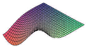
We can use a computer to graph a parametric surface. Below is the graph of the surface

\[\textbf{r}(u,v)= \sin u \hat{\textbf{i}} + \cos v \hat{\textbf{j}} + \text{exp} (2u^{\frac{1}{3}} + 2v^{\frac{1}{3}}) \hat{\textbf{k}}. \]

$alt$

Example $\PageIndex{2}$

Represent the surface

\[z=e^{x} \cos(x-y) \]

parametrically.

Solution

The idea is similar to parametric curves. We just let $x = u$ and $y = v$, to get

\[\textbf{r}(u,v) = u \hat{\textbf{i}} + v \hat{\textbf{j}} + e^{u} \cos(u-v) \hat{\textbf{k}}. \]

$alt$

Example $\PageIndex{3}$

A surface is created by revolving the curve

\[y= \cos x \]

about the x-axis. Find parametric equations for this surface.

Solution

For a fixed value of $x$, we get a circle of radius $\cos x$. Now use polar coordinates (in the yz-plane) to get

\[\textbf{r} (u,v) = u \hat{\textbf{i}} + r \cos v \hat{\textbf{j}} + r \sin v \hat{\textbf{k}}. \]

Since $u = x$ and $\textbf{r} = \cos x$, we can substitute $cos u$ for $\textbf{r}$ in the above equation to get

\[\textbf{r}(u,v) = u \hat{\textbf{i}} + \cos u \cos v \hat{\textbf{j}} + \cos u \sin v \hat{\textbf{k}} .\]

$alt$

Normal Vectors and Tangent Planes

We have already learned how to find a normal vector of a surface that is presented as a function of tow variables, namely find the gradient vector. To find the normal vector to a surface $\textbf{r}(t)$ that is defined parametrically, we proceed as follows.

The partial derivatives

\[\textbf{r}_u (u_0,v_0) \;\;\; \text{and} \;\;\; \textbf{r}_v (u_0,v_0) \]

will lie on the tangent plane to the surface at the point $(u_0,v_0)$. This is true, because fixing one variable constant and letting the other vary, produced a curve on the surface through $(u_0,v_0)$. $\textbf{r}_u (u_0,v_0) $ will be tangent to this curve. The tangent plane contains all vectors tangent to curves passing through the point.

To find a normal vector, we just cross the two tangent vectors.

Example $\PageIndex{4}$

Find the equation of the tangent plane to the surface

\[\textbf{r} (u,v) = (u^2-v^2) \hat{\textbf{i}} + (u+v) \hat{\textbf{j}} + (uv) \hat{\textbf{k}} \]

at the point $(1,2)$.

Solution

We have

\[\textbf{r}_u (u,v) = (2u) \hat{\textbf{i}} + \hat{\textbf{j}} + v \hat{\textbf{k}} \]

\[ \textbf{r}_v (u,v) = (-2v) \hat{\textbf{i}} + \hat{\textbf{j}} + u \hat{\textbf{k}} \]

so that

\[ \textbf{r}_u (1,2) = 2 \hat{\textbf{i}} + \hat{\textbf{j}} + 2 \hat{\textbf{k}} \]

\[ \textbf{r}_v (1,2) = -4 \hat{\textbf{i}} + \hat{\textbf{j}} + \hat{\textbf{k}} \]

\[ \textbf{r}(1,2) = -3 \hat{\textbf{i}} + 3 \hat{\textbf{j}} + 3 \hat{\textbf{k}}. \]

Now cross these vectors together to get

\[\begin{align} r_u \times r_v &= \begin{vmatrix} \hat{\textbf{i}} & \hat{\textbf{j}} &\hat{\textbf{k}} \\ 2 &1 &2 \\ -4 &1 &1 \end{vmatrix} \\ &= - \hat{\textbf{i}} -10 \hat{\textbf{j}} +6 \hat{\textbf{k}}.\end{align}\]

We now have the normal vector and a point $(-3,3,2)$. We use the normal vector-point equation for a plane

\[-1(x+3) - 10(y-3) + 6(z-2)=0 \]

\[-x-10y+6z=-15 \;\;\; \text{or} \;\;\; x+10y-6z=15 .\]

Surface Area

To find the surface area of a parametrically defined surface, we proceed in a similar way as in the case as a surface defined by a function. Instead of projecting down to the region in the xy-plane, we project back to a region in the uv-plane. We cut the region into small rectangles which map approximately to small parallelograms with adjacent defining vectors r_u and r_v. The area of these parallelograms will equal the magnitude of the cross product of r_u and r_v. Finally add the areas up and take the limit as the rectangles get small. This will produce a double integral.

Definition: Area of a Parametric Surface

Let $S$ be a smooth surface defined parametrically by

\[\textbf{r}(u,v) = x(u,v) \hat{\textbf{i}} + y(u,v) \hat{\textbf{j}} + z(u,v) \hat{\textbf{k}} \]

where $u$ and $v$ are contained in a region $\mathbb{R}$. Then the surface area of $S$ is given by

\[SA = \iint_{R} ||r_u \times r_v || \; dudv. \]

Since the magnitude of a cross product involves a square root, the integral in the surface area formula is usually impossible or nearly impossible to evaluate without power series or by approximation techniques.

Example $\PageIndex{5}$

Find the surface area of the surface given by

\[\textbf{r}(u,v)= (v^2) \hat{\textbf{i}} + (u-v) \hat{\textbf{j}} + (u^2) \hat{\textbf{k}} \;\;\; 0 \leq u \leq 2 \;\;\; 1 \leq v \leq 4. \]

Solution

We calculate

\[\textbf{r}_u (u,v) = \hat{\textbf{j}} + 2u \hat{\textbf{k}} \]

\[ \textbf{r}_v (u,v) = (2v) \hat{\textbf{i}} + \hat{\textbf{j}} .\]

The cross product is

\[\begin{align} ||\textbf{r} \times \textbf{r} || &= \begin{vmatrix} \hat{\textbf{i}} & \hat{\textbf{j}} &\hat{\textbf{k}} \\ 0 &1 &2u \\ 2v &-1 &0 \end{vmatrix} \\ &= ||2u \hat{\textbf{i}} + 4uv \hat{\textbf{j}} - 2v \hat{\textbf{k}} || \\ &= 2\sqrt{u^2 + 4u^2v^2+v^2}. \end{align}\]

The surface area formula gives

\[SA=\int_0^2 \int_1^4 2\sqrt{ 4u^2v^2+v^2 } \; dvdu. \]

This integral is probably impossible to compute exactly. Instead, a calculator can be used to obtain a surface area of 70.9.

Larry Green (Lake Tahoe Community College)

Integrated by Justin Marshall.