2.1: Curves

Now that we have a basic understanding of the geometry of \(\mathbb{R}^{n}\), we are in a position to start the study of calculus of more than one variable. We will break our study into three pieces. In this chapter we will consider functions \(f: \mathbb{R} \rightarrow \mathbb{R}^{n}\), in Chapter 3 we will study functions \(f: \mathbb{R}^{n} \rightarrow \mathbb{R}\), and finally in Chapter 4 we will consider the general case of functions \(f: \mathbb{R}^{m} \rightarrow \mathbb{R}^{n}\).

Parametrizations of curves

We begin with some terminology and notation. Given a function \(f: \mathbb{R} \rightarrow \mathbb{R}^{n}\), let

\[ f_{k}(t)=k \text { th coordinate of } f(t) \]

for \(k=1,2, \ldots, n\). We call \(f_{k}: \mathbb{R} \rightarrow \mathbb{R}\) the \(\text { kth coordinate function of } f\). Note that \(f_{k}\) has the same domain as \(f\) and that, for any point \(t\) in the domain of \(f\),

\[ f(t)=\left(f_{1}(t), f_{2}(t), \ldots, f_{n}(t)\right) . \]

If the domain of \(f\) is an interval \(I\), then the range of \(f\), that is, the set

\[ C=\{\mathbf{x}: \mathbf{x}=f(t) \text { for some } t \text { in } I\}, \]

is called a curve with parametrization \(f\). The equation \(\mathbf{x}=f(t)\), where \(\mathbf{x}\) is in \(\mathbb{R}^{n}\), is a vector equation for \(C\) and, writing \(\mathbf{x}=\left(x_{1}, x_{2}, \ldots, x_{n}\right)\), the equations

\[ \begin{align}
x_{1}=f_{1}(t), \nonumber \\
x_{2}=f_{2}(t), \label{} \\
\vdots \quad \vdots \nonumber \\
x_{n}=f_{n}(t), \nonumber
\end{align} \]

are parametric equations for \(C\).

Example \(\PageIndex{1}\)

Consider \(f: \mathbb{R} \rightarrow \mathbb{R}^{2}\) defined by

\[ f(t)=(\cos (t), \sin (t)) \nonumber \]

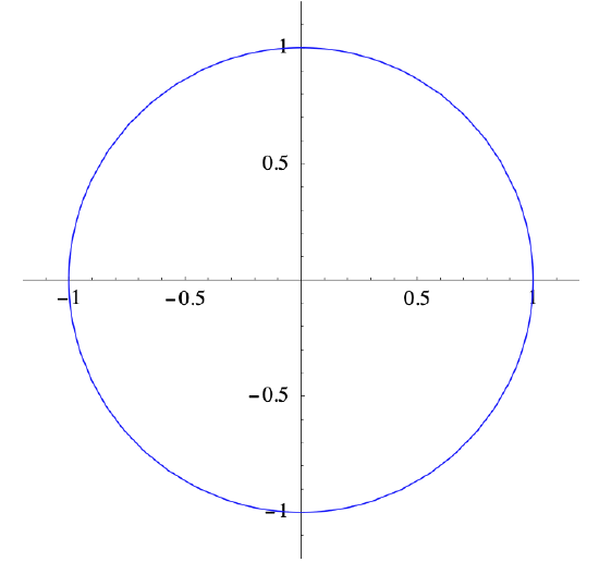
for \(0 \leq t \leq 2 \pi\). Then for every value of \(t\), \(f(t)\) is a point on the circle \(C\) of radius 1 with center at (0,0). Note that \(f(0)=(1,0), f\left(\frac{\pi}{2}\right)=(0,1), f(\pi)=(-1,0), f\left(\frac{3 \pi}{2}\right)=(0,-1) \), and \(f(2 \pi)=(1,0)=f(0)\). In fact, as \(t\) goes from 0 to \(2\pi\), \(f(t)\) traverses \(C\) exactly once in the counterclockwise direction. Thus \(f\) is a parametrization of the unit circle \(C\). If we denote a point in \(\mathbb{R}^{2}\) by \((x,y)\), then

\[ \begin{aligned}
&x=\cos (t), \\
&y=\sin (t),
\end{aligned} \nonumber \]

are parametric equations for \(C\). See Figure 2.1.1. The coordinate functions are

\[ \begin{aligned}
&f_{1}(t)=\cos (t), \\
&f_{2}(t)=\sin (t),
\end{aligned} \]

although we frequently write these as simply

\[ \begin{aligned}
&x(t)=\cos (t), \\
&y(t)=\sin (t).
\end{aligned}\]

Figure \(\PageIndex{1}\): \(f(t)=(\cos (t), \sin (t))\)

Example \(\PageIndex{2}\)

Consider \(g: \mathbb{R} \rightarrow \mathbb{R}^{2}\) defined by

\[ g(t)=(\sin (2 \pi t), \cos (2 \pi t)) \nonumber \]

for \(0 \leq t \leq 2\). Then \(g\) also parametrizes the unit circle \(C\) centered at the origin, the same as \(f\) in the previous example. However, there is a difference: \(g(0)=(0,1), g\left(\frac{1}{4}\right)=(1,0)\), \(g\left(\frac{1}{2}\right)=(0,-1), g\left(\frac{3}{4}\right)=(-1,0), \) and \( g(1)=(0,1)=g(0)\), at which point \(g\) starts to repeat its values. Hence \(g(t)\), starting at (0,1), traverses \(C\) twice in the clockwise direction as \(t\) goes from 0 to 2.

Example \(\PageIndex{3}\)

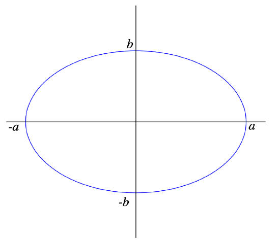
More generally, suppose \(a\), \(b\), and \(\alpha\) are real numbers, with \(a>0\), \(b>0\), and \(\alpha \neq 0\), and let

\[ \begin{aligned}
&x(t)=a \cos (\alpha t), \\
&y(t)=b \sin (\alpha t) .
\end{aligned} \]

Then

\[ \frac{(x(t))^{2}}{a^{2}}+\frac{(y(t))^{2}}{b^{2}}=\cos ^{2}(\alpha t)+\sin ^{2}(\alpha t)=1, \nonumber \]

so \((x(t),y(t))\) is a point on the ellipse \(E\) with equation

\[ \frac{x^{2}}{a^{2}}+\frac{y^{2}}{b^{2}}=1 , \nonumber \]

shown in Figure 2.1.2. Thus the function

\[ f(t)=(a \cos (\alpha t), b \cos (\alpha t)) \nonumber\]

parametrizes the ellipse \(E\), traversing the complete ellipse as \(t\) goes from 0 to \(\left|\frac{2 \pi}{\alpha}\right|\).

Figure \(\PageIndex{2}\): The ellipse \(\frac{x^{2}}{a^{2}}+\frac{y^{2}}{b^{2}}=1\)

Example \(\PageIndex{4}\)

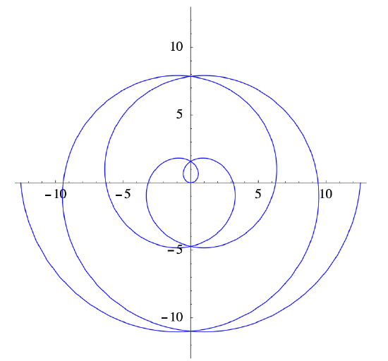
Define \(f: \mathbb{R} \rightarrow \mathbb{R}^{2}\) by

\[ f(t)=(t \cos (t), t \sin (t)) \nonumber \]

for \(-\infty<t<\infty\). Then for negative values of \(t\), \(f(t)\) spirals into the origin as \(t\) increases, while for positive values of \(t\), \(f(t)\) spirals away from the origin. Part of this curve parametrized by \(f\) is shown in Figure 2.1.3.

Figure \(\PageIndex{3}\): The spiral \(f(t)=(t \cos (t), t \sin (t))\) for \(-4 \pi \leq t \leq 4 \pi\)

Example \(\PageIndex{5}\)

Define \(f: \mathbb{R} \rightarrow \mathbb{R}^{2}\) by

\[ f(t)=(3-4 t, 2+3 t) \nonumber \]

for \(-\infty<t<\infty\). Then

\[ f(t)=t(-4,3)+(3,2), \nonumber \]

so \(f\) is a parametrization of the line through the point (3,2) in the direction of (−4,3).

In general, a function \(f: \mathbb{R} \rightarrow \mathbb{R}^{n}\) defined by \(f(t)=t \mathbf{v}+\mathbf{p}\), where \(\mathbf{v} \neq 0\) and \(\mathbf{p}\) are vectors in \(\mathbb{R}^{n}\), parametrizes a line in \(\mathbb{R}^{n}\).

Example \(\PageIndex{6}\)

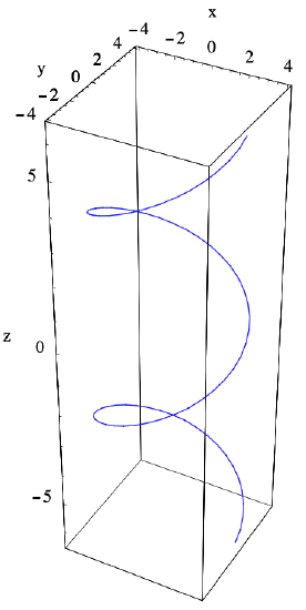
Suppose \(g: \mathbb{R} \rightarrow \mathbb{R}^{3}\) is defined by

\[ g(t)=(4 \cos (t), 4 \sin (t), t) \nonumber \]

for \(-\infty<t<\infty\). If we denote the coordinate functions by

\[ \begin{aligned}
&x(t)=4 \cos (t), \\
&y(t)=4 \sin (t), \\
&z(t)=t ,
\end{aligned} \]

then

\[ (x(t))^{2}+(y(t))^{2}=16 \cos ^{2}(t)+16 \sin ^{2}(t)=16. \nonumber \]

Hence \(g(t)\) always lies on a cylinder of radius 1 centered about the \(z\)-axis. As \(t\) increases, \(g(t)\) rises steadily as it winds around this cylinder, completing one trip around the cylinder over every interval of length \(2\pi\). In other words, \(g\) parametrizes a helix, part of which is shown in Figure 2.1.4.

Figure \(\PageIndex{4}\): The helix \(f(t)=(4 \cos (t), 4 \sin (t), t),-2 \pi \leq t \leq 2 \pi\)

Limits in \(\mathbb{R}^{n}\)

As was the case in one-variable calculus, limits are fundamental for understanding ideas such as continuity and differentiability. We begin with the definition of the limit of a sequence of points in \(\mathbb{R}^{m}\).

Definition \(\PageIndex{1}\)

Let \(\left\{\mathbf{x}_{n}\right\}\) be a sequence of points in \(\mathbb{R}^{m}\). We say that the limit of \(\left\{\mathbf{x}_{n}\right\}\) as \(n\) approaches infinity is \(\mathbf{a}\), written \(\lim _{n \rightarrow \infty} \mathbf{x}_{n}=\mathbf{a}\), if for every \(\epsilon>0\) there is a positive integer \(N\) such that

\[ \left\|\mathbf{x}_{n}-\mathbf{a}\right\|<\epsilon \label{2.1.5}\]

whenever \(n>N\)

Notice that this definition involves only a slight modification of the definition for the limit of a sequence of real numbers, namely, the use of the norm of a vector instead of the absolute value of a real number in (\(\ref{2.1.5}\)). In words, \(\lim _{n \rightarrow \infty} \mathbf{x}_{n}=\mathbf{a}\) if, given any \(\epsilon>0\), we can always find a point in the sequence beyond which all terms of the sequence lie within \(B^{n}(\mathbf{a}, \epsilon)\), the open ball of radius \(\epsilon\) centered at \(\mathbf{a}\).

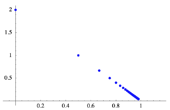
Example \(\PageIndex{7}\)

Suppose

\[ \mathbf{x}_{n}=\left(1-\frac{1}{n}, \frac{2}{n}\right) \nonumber \]

for \(n=1,2,3, \ldots\). Since

\[ \lim _{n \rightarrow \infty}\left(1-\frac{1}{n}\right)=1 \nonumber \]

and

\[ \lim _{n \rightarrow \infty} \frac{2}{n}=0 ,\nonumber \]

we should have

\[ \lim _{n \rightarrow \infty} \mathbf{x}_{n}=(1,0) .\nonumber \]

To verify this, we first note that

\[ \left\|\mathbf{x}_{n}-(1,0)\right\|=\left\|\left(-\frac{1}{n}, \frac{2}{n}\right)\right\|=\sqrt{\frac{1}{n^{2}}+\frac{4}{n^{2}}}=\frac{\sqrt{5}}{n} .\nonumber \]

Hence \(\left\|\mathbf{x}_{n}-(1,0)\right\|<\epsilon\) whenever \(n>\frac{\sqrt{5}}{\epsilon}\). That is, if we let \(N\) be any integer greater than or equal to \(\frac{\sqrt{5}}{\epsilon}\), then \(\left\|\mathbf{x}_{n}-(1,0)\right\|<\epsilon\) whenever \(n > N\), verifying that

\[ \lim _{n \rightarrow \infty} \mathbf{x}_{n}=(1,0) . \nonumber \]

See Figure 2.1.5.

Figure \(\PageIndex{5}\): Points \(\left(1-\frac{1}{n}, \frac{2}{n}\right)\) approaching (1,0)

Put another way, the definition of the limit of a sequence in \(\mathbb{R}^{m}\) says that a sequence \(\left\{\mathbf{x}_{n}\right\}\) in \(\mathbb{R}^{m}\) converges to \(\mathbf{a}\) in \(\mathbb{R}^{m}\) if and only if the sequence of real numbers \(\left\{\left\|\mathbf{x}_{n}-\mathbf{a}\right\|\right\}\) converges to 0. That is, \(\lim _{n \rightarrow \infty} \mathbf{x}_{n}=\mathbf{a}\) if and only if \(\lim _{n \rightarrow \infty}\left\|\mathbf{x}_{n}-\mathbf{a}\right\|=0\). Moreover, if we let \(\mathbf{x}_{n}=\left(x_{n 1}, x_{n 2}, \ldots, x_{n m}\right)\) and \(\mathbf{a}=\left(a_{1}, a_{2}, \ldots, a_{m}\right)\), then

\[\left\|\mathbf{x}_{n}-\mathbf{a}\right\|=\sqrt{\left(x_{n 1}-a_{1}\right)^{2}+\left(x_{n 2}-a_{2}\right)^{2}+\cdots+\left(x_{n m}-a_{m}\right)^{2}},\]

so \(\lim _{n \rightarrow \infty}\left\|\mathbf{x}_{n}-\mathbf{a}\right\|=0\) if and only if

\[ \lim _{n \rightarrow \infty} \sqrt{\left(x_{n 1}-a_{1}\right)^{2}+\left(x_{n 2}-a_{2}\right)^{2}+\cdots+\left(x_{n m}-a_{m}\right)^{2}}=0 . \label{2.1.7} \]

But (\(\ref{2.1.7}\)) can occur only when \(\lim _{n \rightarrow \infty}\left(x_{n k}-a_{k}\right)^{2}=0\) for \(\lim _{n \rightarrow \infty}\left(x_{n k}-a_{k}\right)^{2}=0\). Hence \(\lim _{n \rightarrow \infty} \mathbf{x}_{n}=\mathbf{a}\) if and only if \(\lim _{n \rightarrow \infty} x_{n k}=a_{k}\) for \(k=1,2, \ldots, m\).

Proposition \(\PageIndex{1}\)

Suppose \(\left\{\mathbf{x}_{n}\right\}\) is a sequence in \(\mathbb{R}^{m}\), \(\mathbf{x}_{n}=\left(x_{n 1}, x_{n 2}, \ldots, x_{n m}\right)\), and \(\mathbf{a}= \left(a_{1}, a_{2}, \ldots, a_{m}\right) \). Then \(\lim _{n \rightarrow \infty} \mathbf{x}_{n}=\mathbf{a}\) if and only if \(\lim _{n \rightarrow \infty} x_{n k}=a_{k}\) for \(k=1,2, \ldots, m\).

This proposition tells us that to compute the limit of a sequence in \(\mathbb{R}^{m}\), we need only compute the limit of each coordinate separately, thus reducing the problem of computing limits in \(\mathbb{R}^{m}\) to the problem of finding limits of sequences of real numbers.

Example \(\PageIndex{8}\)

If

\[ \mathbf{x}_{n}=\left(\frac{2-n}{n^{2}}, \sin \left(\frac{1}{n}\right), \cos \left(\frac{3}{n}\right)\right), \nonumber \]

\(n=1,2,3, \ldots\), then

\[ \lim _{n \rightarrow \infty} \mathbf{x}_{n}=\left(\lim _{n \rightarrow \infty} \frac{2-n}{n^{2}}, \lim _{n \rightarrow \infty} \sin \left(\frac{1}{n}\right), \lim _{n \rightarrow \infty} \cos \left(\frac{3}{n}\right)\right)=(0,0,1). \nonumber \]

We may now define the limit of a function \(f: \mathbb{R} \rightarrow \mathbb{R}^{m}\) at a real number \(c\). Notice that the definition is identical to the definition of a limit for a real-valued function \(f: \mathbb{R} \rightarrow \mathbb{R}\).

Definition \(\PageIndex{2}\)

Let \(c\) be a real number, let \(I\) be an open interval containing \(c\), and let \(J=\{t: t \text { is in } I, t \neq c\}\). Suppose \(f: \mathbb{R} \rightarrow \mathbb{R}^{m}\) is defined for all \(t\) in \(J\). Then we say that the limit of \(f(t)\) as \(t\) approaches \(c\) is \(\mathbf{a}\), denoted \(\lim _{t \rightarrow c} f(t)=\mathbf{a}\), if for every sequence of real numbers \(\left\{t_{n}\right\}\) in \(J\),

\[ \lim _{n \rightarrow \infty} f\left(t_{n}\right)=\mathbf{a} \]

whenever \(\lim _{n \rightarrow \infty} t_{n}=c\).

As in one-variable calculus, we may define the limit of \(f(t)\) as \(t\) approaches \(c\) from the right, denoted

\[ \lim _{t \rightarrow c^{+}} f(t), \nonumber \]

by restricting to sequences \(\left\{t_{n}\right\}\) with \(t_{n}>c\) for \(n=1,2,3, \ldots\), and the limit of \(f(t)\) as \(t\) approaches \(c\) from the left, denoted

\[ \lim _{t \rightarrow c^{-}} f(t), \nonumber \]

by restricting to sequences \(\left\{t_{n}\right\}\) with \(t_{n}<c\) for \(n=1,2,3, \ldots\). Moreover, the following useful proposition follows immediately from our definition and the previous proposition.

Proposition \(\PageIndex{2}\)

Suppose \(f: \mathbb{R} \rightarrow \mathbb{R}^{m}\) with

\[ f(t)=\left(f_{1}(t), f_{2}(t), \ldots, f_{m}(t)\right). \nonumber \]

Then for any real number \(c\),

\[ \lim _{t \rightarrow c} f(t)=\left(\lim _{t \rightarrow c} f_{1}(t), \lim _{t \rightarrow c} f_{2}(t), \ldots, \lim _{t \rightarrow c} f_{m}(t)\right).\]

Hence the problem of computing limits for functions \(f: \mathbb{R} \rightarrow \mathbb{R}^{m}\) reduces to the problem of computing limits of the coordinate functions \(f_{k}: \mathbb{R} \rightarrow \mathbb{R}, k=1,2, \ldots, m\), a familiar problem from one-variable calculus. The analogous statements for limits from the right and left also hold.

Example \(\PageIndex{9}\)

If \(f(t)=\left(t^{2}-1, \sin (t), \cos (t)\right)\) is a function from \(\mathbb{R}\) to \(\mathbb{R}^3\), then, for example,

\[ \lim _{t \rightarrow \pi} f(t)=\left(\lim _{t \rightarrow \pi}\left(t^{2}-1\right), \lim _{t \rightarrow \pi} \sin (t), \lim _{t \rightarrow \pi} \cos (t)\right)=\left(\pi^{2}-1,0,-1\right). \nonumber \]

Definitions for continuity also follow the pattern of the related definitions in one variable calculus.

Definition \(\PageIndex{3}\)

Suppose \(f: \mathbb{R} \rightarrow \mathbb{R}^{m}\). We say \(f\) is continuous at a point \(c\) if

\[ \lim _{t \rightarrow c} f(t)=f(c). \]

We say \(f\) is continuous from the right at \(c\) if

\[ \lim _{t \rightarrow c^{+}} f(t)=f(c) \]

and continuous from the left at \(c\) if

\[ \lim _{t \rightarrow c^{-}} f(t)=f(c). \]

We say \(f\) is continuous on an open interval \((a,b)\) if \(f\) is continuous at every point \(c\) in \((a,b)\) and we say \(f\) is continuous on a closed interval \( [a,b] \) if \(f\) is continuous on the open interval \((a,b)\), continuous from the right at \(a\), and continuous from the left at \(b\).

If \(f(t)=\left(f_{1}(t), f_{2}(t), \ldots, f_{m}(t)\right)\), then \(f\) is continuous at a point \(c\) if and only if

\[ \lim _{t \rightarrow c} f(t)=\left(\lim _{t \rightarrow c} f_{1}(t), \lim _{t \rightarrow c} f_{2}(t), \ldots, \lim _{t \rightarrow c} f_{m}(t)=f(c)=\left(f_{1}(c), f_{2}(c), \ldots, f_{m}(c)\right)\right. , \nonumber \]

which is true if and only if \(\lim _{t \rightarrow c} f_{k}(t)=f_{k}(c)\) for \(k=1,2, \ldots, m\). In other words, we have the following useful proposition.

Proposition \(\PageIndex{3}\)

A function \(f: \mathbb{R} \rightarrow \mathbb{R}^{m}\) with \(f(t)=\left(f_{1}(t), f_{2}(t), \ldots, f_{m}(t)\right)\) is continuous at a point \(c\) if and only if the coordinate functions \(f_{1}, f_{2}, \ldots, f_{m}\) are each continuous at \(c\).

Similar statements hold for continuity from the right and from the left.

Example \(\PageIndex{10}\)

The function \(f: \mathbb{R} \rightarrow \mathbb{R}^{3}\) defined by

\[ f(t)=\left(\sin \left(t^{2}\right), t^{3}+4, \cos (t)\right) \nonumber \]

is continuous on the interval \((-\infty, \infty)\) since each of its coordinate functions is continuous on \( (-\infty, \infty)\).