3.1: Geometry, Limits, and Continuity

In this chapter we will study functions \(f: \mathbb{R}^{n} \rightarrow \mathbb{R}\), functions which take vectors for inputs and give scalars for outputs. For example, the function that takes a point in space for input and gives back the temperature at that point is such a function; the function that reports the gross national product of a country is another such function. Note that the domain space of the first example is three-dimensional, while the domain of the latter has, for most countries, thousands of dimensions. As usual, whenever possible we will state our results for an arbitrary \(n\)-dimensional space, although most of our examples will deal with only two or three dimensions.

Level sets and graphs

We begin by considering some geometrical methods for picturing functions of the form \(f: \mathbb{R}^{n} \rightarrow \mathbb{R}\).

Definition \(\PageIndex{1}\)

Given a function \(f: \mathbb{R}^{n} \rightarrow \mathbb{R}\) and a real number \(c\), we call the set

\[ L=\left\{\left(x_{1}, x_{2}, \ldots, x_{n}\right): f\left(x_{1}, x_{2}, \ldots, x_{n}\right)=c\right\} \]

a level set of \(f\) at level \(c\). We also call \(L\) a contour of \(f\). When \(n=2\), we call \(L\) a level curve of \(f\) and when \(n=3\) we call \(L\) a level surface of \(f\). A plot displaying level sets for several different levels is called a contour plot.

Example \(\PageIndex{1}\)

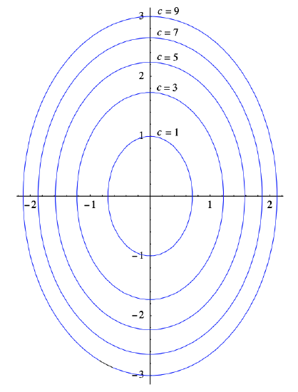
Suppose \(f: \mathbb{R}^{2} \rightarrow \mathbb{R}\) is defined by

\[ f(x, y)=2 x^{2}+y^{2} . \nonumber \]

Given a real number \(c\), the set of all points satisfying

\[ 2 x^{2}+y^{2}=c \nonumber \]

is a level set of \(f\). For \(c<0\), this set is empty; for \(c=0\), it consists of only the point (0,0); for any \(c>0\), the level set is an ellipse with center at (0,0). Hence a contour plot of \(f\), as shown in Figure 3.1.1, consists of concentric ellipses.

Figure \(\PageIndex{1}\): Level curves \(2 x^{2}+y^{2}=c\)

Example \(\PageIndex{2}\)

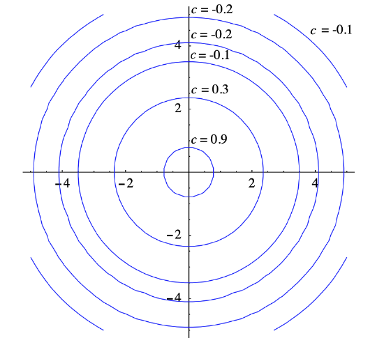
Suppose \(f: \mathbb{R}^{2} \rightarrow \mathbb{R}\) is defined by

\[ f(x, y)=\frac{\sin \left(\sqrt{x^{2}+y^{2}}\right)}{\sqrt{x^{2}+y^{2}}} . \nonumber \]

For any point \((x,y)\) on the circle of radius \(r>0\) centered at the origin, \(f(x,y)\) has the constant value

\[ \frac{\sin (r)}{r} . \nonumber \]

Hence a contour plot of \(f\), like that shown in Figure 3.1.2, consists of concentric circles centered at the origin.

Figure \(\PageIndex{2}\): Level curves \(\frac{\sin \left(\sqrt{x^{2}+y^{2}}\right)}{\sqrt{x^{2}+y^{2}}}=c\)

Example \(\PageIndex{3}\)

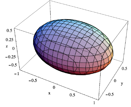
Suppose \(f: \mathbb{R}^{3} \rightarrow \mathbb{R}\) is defined by

\[ f(x, y, z)=x^{2}+2 y^{2}+3 z^{2} . \nonumber \]

The level surface of \(f\) with equation

\[ x^{2}+2 y^{2}+3 z^{2}=1 \nonumber \]

is shown in Figure 3.1.3. Note that, for example, fixing a value \(z_0\) of \(z\) yields the equation

\[ x^{2}+y^{2}=1-3 z_{0}^{2}, \nonumber \]

the equation of an ellipse. This explains why a slice of the level surface shown in Figure 3.1.3 parallel to the \(xy\)-plane is an ellipse. Similarly, slices parallel to the \(xz\)-plane and the \(yz\)-plane are ellipses, which is why this surface is an example of an ellipsoid.

Figure \(\PageIndex{3}\): The level surface \(x^{2}+2 y^{2}+3 z^{2}=1\)

Definition \(\PageIndex{2}\)

Given a function \(f: \mathbb{R}^{n} \rightarrow \mathbb{R}\), we call the set

\[ G=\left\{\left(x_{1}, x_{2}, \ldots, x_{n}, x_{n+1}\right): x_{n+1}=f\left(x_{1}, x_{2}, \ldots, x_{n}\right)\right\} \]

the graph of \(f\).

Note that the graph \(G\) of a function \(f: \mathbb{R}^{n} \rightarrow \mathbb{R}\) is in \(R^{n+1}\). As a consequence, we can picture \(G\) only if \(n=1\), in which case \(G\) is a curve as studied in single-variable calculus, or \(n=2\), in which case \(G\) is a surface in \(\mathbb{R}^{3}\).

Example \(\PageIndex{4}\)

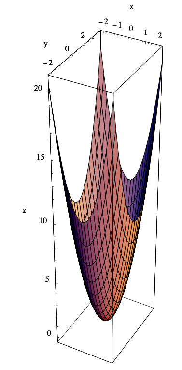
Consider the function \(f: \mathbb{R}^{2} \rightarrow \mathbb{R}\) defined by

\[ f(x, y)=2 x^{2}+y^{2} . \nonumber \]

The graph of \(f\) is then the set of all points \((x,y,z)\) in \(\mathbb{R}^{3}\) which satisfy the equation \(z=2 x^{2}+y^{2}\). One way to picture the graph of \(f\) is to imagine raising the level curves in Figure 3.1.1 to their respective heights above the \(xy\)-plane, creating the surface in \(\mathbb{R}^{3}\) shown in Figure 3.1.4. Another way to picture the graph is to consider slices of the graph lying above a grid of lines parallel to the axes in the \(xy\)-plane. For example, for a fixed value of \(x\), say \(x_0\), the set of points satisfying the equation \(z=2 x_{0}^{2}+y^{2}\) is a parabola lying above the line \(x=x_0\). Similarly, fixing a value \(y_0\) of \(y\) yields the parabola \(z=2 x^{2}+y_{0}\) lying above the line \(y=y_0\). If we draw these parabolas for numerous lines of the form \(x=x_0\) and \(y=y_0\), we obtain a wire-frame of the graph. The graph shown in Figure 3.1.4 was obtained by filling in the surface patches of a wire-frame mesh, the outline of which is visible on the surface. This surface is an example of a paraboloid.

Figure \(\PageIndex{4}\): The paraboloid \(z=2 x^{2}+y^{2}\)

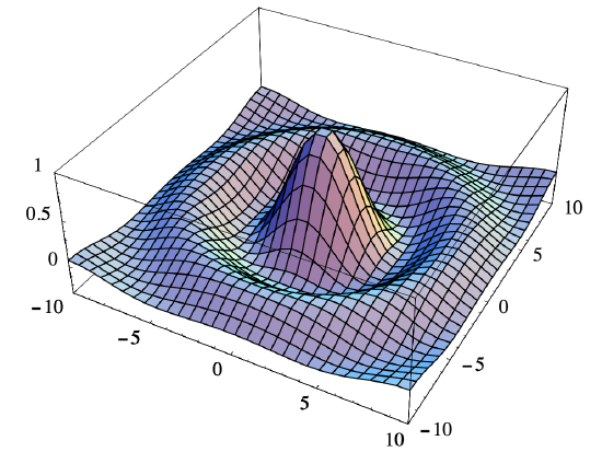
Example \(\PageIndex{5}\)

Although the graphs of many functions may be sketched reasonably well by hand using the ideas of the previous example, for most functions a good picture of its graph requires either computer graphics or considerable artistic skill. For example, consider the graph of

\[ f(x, y)=\frac{\sin \left(\sqrt{x^{2}+y^{2}}\right)}{\sqrt{x^{2}+y^{2}}} . \nonumber \]

Using the contour plot, we can imagine how the graph of \(f\) oscillates as we move away from the origin, the level circles of the contour plot rising and falling with the oscillations of

\[ \frac{\sin (r)}{r} , \nonumber \]

where \(r=\sqrt{x^{2}+y^{2}}\). Equivalently, the slice of the graph above any line through the origin will be the graph of

\[ z=\frac{\sin (r)}{r} . \nonumber \]

This should give you a good idea what the graph of \(f\) looks like, but, nevertheless, most of us could not produce the picture of Figure 3.1.5 without the aid of a computer. Notice that although \(f\) is not defined at (0,0), it appears that \(f(x,y)\) approaches 1 as \((x,y)\) approaches 0. This is in fact true, a consequence of the fact that

\[ \lim _{r \rightarrow 0} \frac{\sin (r)}{r}=1 . \nonumber \]

We will return to this example after we have introduced limits and continuity.

Figure \(\PageIndex{5}\): Graph of \(f(x, y)=\frac{\sin \left(\sqrt{x^{2}+y^{2}}\right)}{\sqrt{x^{2}+y^{2}}}\)

Limits and continuity

By now the following two definitions should look familiar.

Definition \(\PageIndex{3}\)

Let \(\mathbf{a}\) be a point in \(\mathbb{R}^{n}\) and let \(O\) be the set of all points in the open ball of radius \(r>0\) centered at \(\mathbf{c}\) except \(\mathbf{c}\) itself. That is,

\[ O=\left\{\mathbf{x}: \mathbf{x} \text { is in } B^{n}(\mathbf{c}, r), \mathbf{x} \neq \mathbf{c}\right\} . \]

Suppose \(f: \mathbb{R}^{n} \rightarrow \mathbb{R}\) is defined for all \(\mathbf{x}\) in \(O\). We say the limit of \(f(\mathbf{x})\) as \(x\) approaches \(\mathbf{c}\) is \(L\), written \(\lim _{\mathbf{x} \rightarrow \mathbf{c}} f(\mathbf{x})=L\), if for every sequence of points \(\left\{\mathbf{x}_{m}\right\}\) in \(O\),

\[ \lim _{m \rightarrow \infty} f\left(\mathbf{x}_{m}\right)=L \]

whenever \(\lim _{m \rightarrow \infty} \mathbf{x}_{m}=\mathbf{c}\).

Definition \(\PageIndex{4}\)

Suppose \(f: \mathbb{R}^{n} \rightarrow \mathbb{R}\) is defined for all \(\mathbf{x}\) in some open ball \(B^{n}(\mathbf{c}, r), r>0\). We say \(f\) is continuous at \(\mathbf{c}\) if

\[ \lim _{\mathbf{x} \rightarrow \mathbf{c}} f(\mathbf{x})=f(\mathbf{c}) . \]

The following basic properties of limits follow immediately from the analogous properties for limits of sequences.

Proposition \(\PageIndex{1}\)

Suppose \(f: \mathbb{R}^{n} \rightarrow \mathbb{R}\) and \(g: \mathbb{R}^{n} \rightarrow \mathbb{R}\) with

\[ \lim _{\mathbf{x} \rightarrow \mathbf{c}} f(\mathbf{x})=L \nonumber \]

and

\[ \lim _{\mathbf{x} \rightarrow \mathbf{c}} g(\mathbf{x})=M. \nonumber \]

Then

\[ \begin{align}
\lim _{\mathbf{x} \rightarrow \mathbf{c}}(f(\mathbf{x})+g(\mathbf{x}))=L+M, \label{3.1.6} \\
\lim _{\mathbf{x} \rightarrow \mathbf{c}}(f(\mathbf{x})-g(\mathbf{x}))=L-M, \label{3.1.7} \\
\lim _{\mathbf{x} \rightarrow \mathbf{c}} f(\mathbf{x}) g(\mathbf{x})=L M, \label{3.1.8} \\
\lim _{\mathbf{x} \rightarrow \mathrm{c}} \frac{f(\mathbf{x})}{g(\mathbf{x})}=\frac{L}{M}, \label{3.1.9}
\end{align} \]

and

\[ \lim _{\mathbf{x} \rightarrow \mathbf{c}} k f(\mathbf{x})=k L \label{3.1.10} \]

for any scalar \(k\).

Now suppose \(f: \mathbb{R}^{n} \rightarrow \mathbb{R}\), \(h: \mathbb{R} \rightarrow \mathbb{R}\),

\[ \lim _{\mathbf{x} \rightarrow \mathbf{c}} f(\mathbf{x})=L , \]

and \(h\) is continuous at \(L\). Then for any sequence \(\left\{\mathbf{x}_{m}\right\}\) in \(\mathbb{R}^n\) with

\[ \lim _{m \rightarrow \infty} \mathbf{x}_{m}=\mathbf{c} , \]

we have

\[ \lim _{m \rightarrow \infty} f\left(\mathbf{x}_{m}\right)=L , \]

and so

\[ \lim _{m \rightarrow \infty} h\left(f\left(\mathbf{x}_{m}\right)\right)=h(L) \]

by the continuity of \(h\) at \(L\). Thus we have the following result about compositions of functions.

Proposition \(\PageIndex{2}\)

If \(f: \mathbb{R}^{n} \rightarrow \mathbb{R}\), \(h: \mathbb{R} \rightarrow \mathbb{R}\),

\[ \lim _{\mathbf{x} \rightarrow \mathbf{c}} f(\mathbf{x})=L , \nonumber \]

and \(h\) is continuous at \(L\), then

\[ \lim _{\mathbf{x} \rightarrow \mathbf{c}} h \circ f(\mathbf{x})=\lim _{\mathbf{x} \rightarrow \mathbf{c}} h(f(\mathbf{x}))=h(L) . \label{3.1.15} \]

Example \(\PageIndex{6}\)

Suppose we define \(f: \mathbb{R}^{n} \rightarrow \mathbb{R}\) by

\[ f\left(x_{1}, x_{2}, \ldots, x_{n}\right)=x_{k} , \nonumber \]

where \(k\) is a fixed integer between 1 and \(n\). If \(\mathbf{a}=\left(a_{1}, a_{2}, \ldots, a_{n}\right)\) is a point in \(\mathbb{R}^n\) and \(\lim _{m \rightarrow \infty} \mathbf{x}_{m}=\mathbf{a}\), then

\[ \lim _{m \rightarrow \infty} f\left(\mathbf{x}_{m}\right)=\lim _{m \rightarrow \infty} x_{m k}=a_{k}, \nonumber \]

where \(x_{mk}\) is the \(k\)th coordinate of \(\mathbf{x}_m\). Thus

\[ \lim _{\mathbf{x} \rightarrow \mathbf{a}} f(\mathbf{x})=a_{k} . \nonumber \]

This result is a basic building block for the examples that follow. For a particular example, if \(f(x, y)=x,\) then

\[ \lim _{(x, y) \rightarrow(2,3)} f(x, y)=\lim _{(x, y) \rightarrow(2,3)} x=2 . \nonumber \]

Example \(\PageIndex{7}\)

If we define \(f: \mathbb{R}^{3} \rightarrow \mathbb{R}\) by

\[ f(x, y, z)=x y z , \nonumber \]

then, using (\(\ref{3.1.8}\)) in combination with the previous example,

\begin{aligned}
\lim _{(x, y, z) \rightarrow(a, b, c)} f(x, y, z) &=\lim _{(x, y, z) \rightarrow(a, b, c)} x y z \\
&=\left(\lim _{(x, y, z) \rightarrow(a, b, c)} x\right)\left(\lim _{(x, y, z) \rightarrow(a, b, c)} y\right)\left(\lim _{(x, y, z) \rightarrow(a, b, c)} z\right) \\
&=a b c .
\end{aligned}

for any point \((a,b,c)\) in \(\mathbb{R}^{3}\). For example,

\[ \lim _{(x, y, z) \rightarrow(3,2,1)} f(x, y, z)=\lim _{(x, y, z) \rightarrow(3,2,1)} x y z=(3)(2)(1)=6 . \nonumber \]

Example \(\PageIndex{8}\)

Combining the previous examples with (\(\ref{3.1.6}\)), (\(\ref{3.1.7}\)), (\(\ref{3.1.8}\)), and (\(\ref{3.1.10}\)), we have

\begin{aligned}
\lim _{(x, y, z) \rightarrow(2,1,3)}\left(x y^{2}+3 x y z-6 x z\right)=(&\left.\lim _{(x, y, z) \rightarrow(2,1,3)} x\right)\left(\lim _{(x, y, z) \rightarrow(2,1,3)} y\right)\left(\lim _{(x, y, z) \rightarrow(2,1,3)} y\right) \\
&+3\left(\lim _{(x, y, z) \rightarrow(2,1,3)} x\right)\left(\lim _{(x, y, z) \rightarrow(2,1,3)} y\right)\left(\lim _{(x, y, z) \rightarrow(2,1,3)} z\right) \\
&-6\left(\lim _{(x, y, z) \rightarrow(2,1,3)} x\right)\left(\lim _{(x, y, z) \rightarrow(2,1,3)} z\right) \\
=&(2)(1)(1)+(3)(2)(1)(3)-(6)(2)(3) \\
=&-16 .
\end{aligned}

The last three examples are all examples of polynomials in several variables. In general, a function \(f: \mathbb{R}^{n} \rightarrow \mathbb{R}\) of the form

\[ f\left(x_{1}, x_{2}, \ldots, x_{n}\right)=a x_{1}^{i_{1}} x_{2}^{i_{2}} \cdots x_{n}^{i_{n}} , \nonumber \]

where \(a\) is a scalar and \(i_{1}, i_{2}, \ldots, i_{n}\) are nonnegative integers, is called a monomial. A function which is a sum of monomials is called a polynomial. The following proposition is a consequence of the previous examples and (\(\ref{3.1.6}\)), (\(\ref{3.1.7}\)), (\(\ref{3.1.8}\)), and (\(\ref{3.1.10}\)).

Proposition \(\PageIndex{3}\)

If \(f: \mathbb{R}^{n} \rightarrow \mathbb{R}\) is a polynomial, then for any point \(\mathbf{c}\) in \(\mathbb{R}^n\),

\[ \lim _{\mathbf{x} \rightarrow \mathbf{c}} f(\mathbf{x})=f(\mathbf{c}) . \]

In other words, \(f\) is continuous at every point \(\mathbf{c}\) in \(\mathbb{R}^n\).

If \(g\) and \(h\) are both polynomials, then we call the function

\[ f(\mathbf{x})=\frac{g(\mathbf{x})}{h(\mathbf{x})} \]

a rational function. The next proposition is a consequence of the previous theorem and (\(\ref{3.1.9}\)).

Proposition \(\PageIndex{4}\)

If \(f: \mathbb{R}^{n} \rightarrow \mathbb{R}\) is a rational function defined at \(\mathbf{c}\), then

\[ \lim _{\mathbf{x} \rightarrow \mathbf{c}} f(\mathbf{x})=f(\mathbf{c}) . \label{3.1.18} \]

In other words, \(f\) is continuous at every point \(\mathbf{c}\) in its domain.

Example \(\PageIndex{9}\)

Since

\[ f(x, y, z)=\frac{x^{2} y+3 x y z^{2}}{4 x^{2}+3 z^{2}} \nonumber \]

is a rational function, we have, for example,

\[ \lim _{(x, y, z) \rightarrow(2,1,3)} f(x, y, z)=\lim _{(x, y, z) \rightarrow(2,1,3)} \frac{x^{2} y+3 x y z^{2}}{4 x^{2}+3 z^{2}}=\frac{4+54}{16+27}=\frac{58}{43} . \nonumber \]

Example \(\PageIndex{10}\)

Combining (\(\ref{3.1.18}\)) with (\(\ref{3.1.15}\)), we have

\[ \begin{aligned}
\lim _{(x, y, z) \rightarrow(1,2,1)} \log \left(\frac{1}{x^{2}+y^{2}+z^{2}}\right) &=\log \left(\lim _{(x, y, z) \rightarrow(1,2,1)} \frac{1}{x^{2}+y^{2}+z^{2}}\right) \\
&=\log \left(\frac{1}{6}\right) \\
&=-\log (6) .
\end{aligned} \]

From the continuity of the square root function and our result above about the continuity of polynomials, we may conclude that the function \(f: \mathbb{R}^{n} \rightarrow \mathbb{R}\) defined by

\[ f\left(x_{1}, x_{2}, \ldots, x_{n}\right)=\left\|\left(x_{1}, x_{2}, \ldots, x_{n}\right)\right\|=\sqrt{x_{1}^{2}+x_{2}^{2}+\cdots+x_{n}^{2}} \nonumber \]

is a continuous function. This fact is useful in computing some limits, particularly in combination with the fact that for any point \(\mathbf{x}=\left(x_{1}, x_{2}, \ldots, x_{n}\right)\) in \(\mathbb{R}^n\),

\[ \|\mathbf{x}\|=\sqrt{x_{1}^{2}+x_{2}^{2}+\cdots+x_{n}^{2}} \geq \sqrt{x_{k}^{2}}=\left|x_{k}\right| \label{3.1.19} \]

for any \(k=1,2, \ldots, n\).

Example \(\PageIndex{11}\)

Suppose \(f: \mathbb{R}^{2} \rightarrow \mathbb{R}\) is defined by

\[ f(x, y)=\frac{x^{2} y}{x^{2}+y^{2}} . \nonumber \]

Although \(f\) is a rational function, we cannot use (\(\ref{3.1.18}\)) to compute

\[ \lim _{(x, y) \rightarrow(0,0)} f(x, y) \nonumber \]

since \(f\) is not defined at (0,0). However, if we let \(\mathbf{x}=(x, y)\), then, using (\(\ref{3.1.19}\)),

\[ |f(x, y)|=\left|\frac{x^{2} y}{x^{2}+y^{2}}\right|=\frac{|x|^{2}|y|}{\left|x^{2}+y^{2}\right|}=\frac{|x|^{2}|y|}{\|\mathbf{x}\|^{2}} \leq \frac{\|\mathbf{x}\|^{2}\|\mathbf{x}\|}{\|\mathbf{x}\|^{2}}=\|\mathbf{x}\| . \nonumber \]

Now

\[ \lim _{(x, y) \rightarrow(0,0)}\|\mathbf{x}\|=0 , \nonumber \]

so

\[ \lim _{(x, y) \rightarrow(0,0)}|f(x, y)|=0 . \nonumber \]

Hence

\[ \lim _{(x, y) \rightarrow(0,0)} f(x, y)=\lim _{(x, y) \rightarrow(0,0)} \frac{x^{2} y}{x^{2}+y^{2}}=0 . \nonumber \]

See Figure 3.1.6.

Figure \(\PageIndex{6}\): Graph of \(f(x, y)=\frac{x^{2} y}{x^{2}+y^{2}}\)

Recall that for a function \(\varphi: \mathbb{R} \rightarrow \mathbb{R}\),

\[ \lim _{t \rightarrow c} \varphi(t)=L \nonumber \]

if and only if both

\[ \lim _{t \rightarrow c^{-}} \varphi(t)=L \nonumber \]

and

\[ \lim _{t \rightarrow c^{+}} \varphi(t)=L . \nonumber \]

In particular, if the one-sided limits do not agree, we may conclude that the limit does not exist. Similar reasoning may be applied to a function \(f: \mathbb{R}^{n} \rightarrow \mathbb{R}\), the difference being that there are infinitely many different curves along which the variable \(\mathbf{x}\) might approach a given point \(\mathbf{c}\) in \(\mathbb{R}^n\), as opposed to only the two directions of approach in \(\mathbb{R}\). As a consequence, it is not possible to establish the existence of a limit with this type of argument. Nevertheless, finding two ways to approach \(\mathbf{c}\) which yield different limiting values is sufficient to show that the limit does not exist.

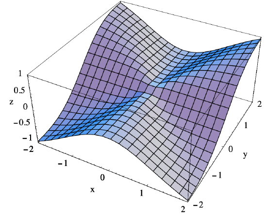
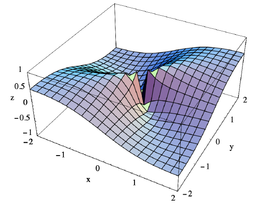
Example \(\PageIndex{12}\)

Suppose \(g: \mathbb{R}^{2} \rightarrow \mathbb{R}\) is defined by

\[ g(x, y)=\frac{x y}{x^{2}+y^{2}} . \nonumber \]

If we define \(\alpha: \mathbb{R}^{2} \rightarrow \mathbb{R}\) by \(\alpha(t)=(t, 0)\), then

\[ \lim _{t \rightarrow 0} \alpha(t)=\lim _{t \rightarrow 0}(t, 0)=(0,0) \nonumber \]

and

\[ \lim _{t \rightarrow 0} g(\alpha(t))=\lim _{t \rightarrow 0} f(t, 0)=\lim _{t \rightarrow 0} \frac{0}{t^{2}}=0 . \nonumber \]

Now \(\alpha\) is a parametrization of the \(x\)-axis, so the previous limit computation says that \(g(x,y)\) approaches 0 as \((x,y)\) approaches (0,0) along the \(x\)-axis. However, if we define \(\beta: \mathbb{R} \rightarrow \mathbb{R}^{2}\) by \(\beta(t)=(t, t)\), then \(\beta\) parametrizes the line \(x=y\),

\[ \lim _{t \rightarrow 0} \beta(t)=\lim _{t \rightarrow 0}(t, t)=(0,0) , \nonumber \]

and

\[ \lim _{t \rightarrow 0} g(\beta(t))=\lim _{t \rightarrow 0} f(t, t)=\lim _{t \rightarrow 0} \frac{t^{2}}{2 t^{2}}=\frac{1}{2} . \nonumber \]

Hence \(g(x,y)\) approaches \(\frac{1}{2}\) as \((x,y)\) approaches (0,0) along the line \(x=y\). Since these two limits are different, we may conclude that \(g(x,y)\) does not have a limit as \((x,y)\) approaches (0,0). Note that \(g\) in this example and \(f\) in the previous example are very similar functions, although our limit calculations show that their behavior around (0,0) differs significantly. In particular, \(f\) has a limit as \((x,y)\) approaches (0,0), whereas \(g\) does not. This may be

seen by comparing the graph of \(g\) in Figure 3.1.7, which has a tear at the origin, with that of \(f\) in Figure 3.1.6.

Figure \(\PageIndex{7}\): Graph of \(g(x, y)=\frac{x y}{x^{2}+y^{2}}\)

The next proposition lists some basic properties of continuous functions, all of which follow immediately from the similar list of properties of limits.

Proposition \(\PageIndex{5}\)

Suppose \(f: \mathbb{R}^{n} \rightarrow \mathbb{R}\) and \(g: \mathbb{R}^{n} \rightarrow \mathbb{R}\) are both continuous at \(\mathbf{c}\). Then the functions with values at \(\mathbf{x}\) given by

\[ \begin{align}
f(\mathbf{x})+g(\mathbf{x}), \label{3.1.20} \\
f(\mathbf{x})-g(\mathbf{x}), \label{3.1.21} \\
f(\mathbf{x}) g(\mathbf{x}), \label{3.1.22} \\
\frac{f(\mathbf{x})}{g(\mathbf{x})} \label{3.1.23}
\end{align} \]

(provided \(g(\mathbf{c}) \neq 0\)), and

\[ k f(\mathbf{x}), \label{3.1.24} \]

where \(k\) is any scalar, are all continuous at \(\mathbf{c}\).

From the result above about the limit of a composition of two functions, we have the following proposition.

Proposition \(\PageIndex{6}\)

If \(f: \mathbb{R}^{n} \rightarrow \mathbb{R}\) is continuous at \(\mathbf{c}\) and \(\varphi: \mathbb{R} \rightarrow \mathbb{R}\) is continuous at \(f(\mathbf{c})\), then \(\varphi \circ f\) is continuous at \(\mathbf{c}\).

Example \(\PageIndex{13}\)

Since the function \(\varphi(t)=\sin (t)\) is continuous for all \(t\) and the function

\[ f(x, y, z)=\sqrt{x^{2}+y^{2}+z^{2}} \nonumber \]

is continuous at all points \((x,y,z)\) in \(\mathbb{R}^3\), the function

\[ g(x, y, z)=\sin \left(\sqrt{x^{2}+y^{2}+z^{2}}\right) \nonumber \]

is continuous at all points \((x,y,z)\) in \(\mathbb{R}^3\).

Example \(\PageIndex{14}\)

Since the function

\[ h(x, y)=\sin \left(\sqrt{x^{2}+y^{2}}\right) \nonumber \]

is continuous for all \((x,y)\) in \(\mathbb{R}^2\) (same argument as in the previous example) and the function

\[ g(x, y)=\sqrt{x^{2}+y^{2}} \nonumber \]

is continuous for all \((x,y)\) in \(\mathbb{R}^2\), the function

\[ f(x, y)=\frac{\sin \left(\sqrt{x^{2}+y^{2}}\right)}{\sqrt{x^{2}+y^{2}}} \nonumber \]

is, using (\(\ref{3.1.23}\)), continuous at every point \((x, y) \neq(0,0)\) in \(\mathbb{R}^{2}\). Moreover, if we let \(\mathbf{x}=(x, y)\), then

\[ \lim _{(x, y) \rightarrow(0,0)} f(x, y)=\lim _{(x, y) \rightarrow(0,0)} \frac{\sin \left(\sqrt{x^{2}+y^{2}}\right)}{\sqrt{x^{2}+y^{2}}}=\lim _{(x, y) \rightarrow(0,0)} \frac{\sin (\|\mathbf{x}\|)}{\|\mathbf{x}\|}=\lim _{r \rightarrow 0} \frac{\sin (r)}{r}=1 . \nonumber \]

Hence the discontinuity at (0,0) is removable. That is, if we define

\[ g(x, y)= \begin{cases}\frac{\sin \left(\sqrt{x^{2}+y^{2}}\right)}{\sqrt{x^{2}+y^{2}}}, & \text { if }(x, y) \neq(0,0), \\ 1, & \text { if }(x, y)=(0,0),\end{cases} \nonumber \]

then \(g\) is continuous for all \((x,y)\) in \(\mathbb{R}^2\).

Open and closed sets

In single-variable calculus we talk about a function being continuous not just at a point, but on an open interval, meaning that the function is continuous at every point in the open interval. Similarly, we need to generalize the definition of continuity of a function \(f: \mathbb{R}^{n} \rightarrow \mathbb{R}\) from that of continuity at a point in \(\mathbb{R}^n\) to the idea of a function being continuous on a set in \(\mathbb{R}^n\). Now the condition for a function \(f\) to be continuous at a point \(\mathbf{c}\) requires that \(f\) be defined on some open ball containing \(\mathbf{c}\). Hence, in order to say that \(f\) is continuous at every point in some set \(U\), it is necessary that, given any point \(\mathbf{u}\) in \(U\), \(f\) be defined on some open ball containing \(\mathbf{u}\). This provides the motivation for the following definition.

Definition \(\PageIndex{5}\)

We say a set of points \(U\) in \(\mathbb{R}^n\) is open if whenever \(\mathbf{u}\) is a point in \(U\), there exists a real number \(r>0\) such that the open ball \(B^{n}(\mathbf{u}, r)\) lies entirely within \(U\). We say a set of points \(C\) in \(\mathbb{R}^n\) is closed if the set of all points in \(\mathbb{R}^n\) which do not lie in \(C\) form an open set.

Example \(\PageIndex{15}\)

\(\mathbb{R}^n\) is itself an open set.

Example \(\PageIndex{16}\)

Any open ball in \(\mathbb{R}^n\) is an open set. In particular, any open interval in \(\mathbb{R}\) is an open set. To see why, consider an open ball \(B^{n}(\mathbf{a}, r)\) in \(\mathbb{R}^n\). Given a point \(\mathbf{y}\) in \(B^{n}(\mathbf{a}, r)\), let \(s\) be the smaller of \(\|\mathbf{y}-\mathbf{a}\|\) (the distance from \(\mathbf{y}\) to the center of the ball) and \(r-\|\mathbf{y}-\mathbf{a}\|\) (the distance from \(\mathbf{y}\) to the edge of the ball). Then \(B^{n}(\mathbf{y}, s)\) is an open ball which lies entirely within \(B^{n}(\mathbf{a}, r)\). Hence \(B^{n}(\mathbf{a}, r)\) is an open set.

Example \(\PageIndex{17}\)

Any closed ball in \(\mathbb{R}^n\) is a closed set. In particular, any closed interval in \(\mathbb{R}\) is a closed set. To see why, consider a closed ball \(\bar{B}^{n}(\mathbf{a}, r)\). Given a point \(\mathbf{y}\) not in \(\bar{B}^{n}(\mathbf{a}, r)\), let \(s=\|\mathbf{y}-\mathbf{a}\|-r\), the distance from \(\mathbf{y}\) to the edge of \(\bar{B}^{n}(\mathbf{a}, r)\). Then \(B^{n}(\mathbf{y}, s)\) is an open ball which lies entirely outside of \(\bar{B}^{n}(\mathbf{x}, r)\). Hence \(\bar{B}^{n}(\mathbf{x}, r)\) is a closed set.

Example \(\PageIndex{18}\)

Given real numbers \(a_{1}<b_{1}, a_{2}<b_{2}, \ldots, a_{n}<b_{n}\), we call the set

\[ U=\left\{\left(x_{1}, x_{2}, \ldots, x_{n}\right): a_{i}<x_{i}<b_{i}, i=1,2, \ldots, n\right\} \nonumber \]

an open rectangle in \(\mathbb{R}^n\) and the set

\[ C=\left\{\left(x_{1}, x_{2}, \ldots, x_{n}\right): a_{i} \leq x_{i} \leq b_{i}, i=1,2, \ldots, n\right\} \nonumber \]

a closed rectangle in \(\mathbb{R}^n\). An argument similar to that in the previous example shows that \(U\) is an open set and \(C\) is a closed set.

Definition \(\PageIndex{6}\)

We say a function \(f: \mathbb{R}^{n} \rightarrow \mathbb{R}\) is continuous on an open set \(U\) if \(f\) is continuous at every point \(u\) in \(U\).

Example \(\PageIndex{19}\)

The function

\[ f(x, y, z)=\frac{3 x y z-6 x}{x^{2}+y^{2}+z^{2}+1} \nonumber \]

is continuous on \(\mathbb{R}^3\).

Example \(\PageIndex{20}\)

The functions

\[ f(x, y)= \begin{cases}\frac{x^{2} y}{x^{2}+y^{2}}, & \text { if }(x, y) \neq(0,0), \\ 0, & \text { if }(x, y)=(0,0), \end{cases} \nonumber \]

and

\[ g(x, y)= \begin{cases}\frac{\sin \left(\sqrt{x^{2}+y^{2}}\right)}{\sqrt{x^{2}+y^{2}}}, & \text { if }(x, y) \neq(0,0), \\ 1, & \text { if }(x, y)=(0,0),\end{cases} \nonumber \]

are, from our work in previous examples, continuous on \(\mathbb{R}^2\).

Example \(\PageIndex{21}\)

The function

\[ g(x, y)=\frac{x y}{x^{2}+y^{2}} \nonumber \]

is continuous on the open set

\[ U=\big\{(x, y):(x, y) \neq(0,0)\big\}. \nonumber \]

Note that in this case it is not possible to define \(g\) at \((0,0)\) in such a way that the resulting function is continuous at \((0,0),\) a consequence of our work above showing that \(g\) does not have a limit as \((x,y)\) approaches \((0,0).\)

Example \(\PageIndex{22}\)

The function

\[ f(x, y)=\log (x y) \nonumber \]

is continuous on the open set

\[ U=\big\{(x, y): x>0 \text { and } y>0\big\}. \nonumber \]