3.2: Directional Derivatives and the Gradient

For a function \(\varphi: \mathbb{R} \rightarrow \mathbb{R}\), the derivative at a point \(c\), that is,

\[ \varphi^{\prime}(c)=\lim _{h \rightarrow 0} \frac{\varphi(c+h)-\varphi(c)}{h}, \label{3.2.1} \]

is the slope of the best affine approximation to \(\varphi\) at \(c\). We may also regard it as the slope of the graph of \(\varphi\) at \((c, \varphi(c))\), or as the instantaneous rate of change of \(\varphi(x)\) with respect to \(x\) when \(x=c\). As a prelude to finding the best affine approximations for a function \(f: \mathbb{R}^{n} \rightarrow \mathbb{R}\), we will first discuss how to generalize (\(\ref{3.2.1}\)) to this setting using the ideas of slopes and rates of change for our motivation.

Directional derivatives

Example \(\PageIndex{1}\)

Consider the function \(f: \mathbb{R}^{2} \rightarrow \mathbb{R}\) defined by

\[ f(x, y)=4-2 x^{2}-y^{2} , \nonumber \]

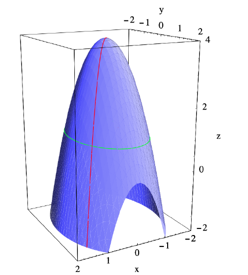
the graph of which is pictured in Figure 3.2.1. If we imagine a bug moving along this surface, then the slope of the path encountered by the bug will depend both on the bug’s position and the direction in which it is moving. For example, if the bug is above the point (1,1) in the \(xy\)-plane, moving in the direction of the vector \(\mathbf{v}=(-1,-1)\) will cause it to head directly towards the top of the graph, and thus have a steep rate of ascent, whereas moving in the direction of \(-\mathbf{v}=(1,1)\) would cause it to descend at a fast rate. These two possibilities are illustrated by the red curve on the surface in Figure 3.2.1. For another example, heading around the surface above the ellipse

\[ 2 x^{2}+y^{2}=3 \nonumber \]

in the \(xy\)-plane, which from (1,1) means heading initially in the direction of the vector \(\mathbf{w}=(-1,2)\), would lead the bug around the side of the hill with no change in elevation, and hence a slope of 0. This possibility is illustrated by the green curve on the surface in Figure 3.2.1. Thus in order to talk about the slope of the graph of \(f\) at a point, we must specify a direction as well.

Figure \(\PageIndex{1}\): Graph of \(f(x)=4-2 x^{2}-y^{2}\)

For example, suppose the bug moves in the direction of \(\mathbf{v}\). If we let

\[ \mathbf{u}=-\frac{1}{\sqrt{2}}(1,1) , \nonumber \]

the direction of \(\mathbf{v}\), then, letting \(\mathbf{c}=(1,1)\),

\[ \frac{f(\mathbf{c}+h \mathbf{u})-f(\mathbf{c})}{h} \nonumber \]

would, for any \(h>0\), represent an approximation to the slope of the graph of \(f\) at (1,1) in the direction of \(\mathbf{u}\). As in single-variable calculus, we should expect that taking the limit as \(h\) approaches 0 should give us the exact slope at (1,1) in the direction of \(\mathbf{u}\). Now

\[ \begin{aligned}
f(\mathbf{c}+h \mathbf{u})-f(\mathbf{c}) &=f\left(1-\frac{h}{\sqrt{2}}, 1-\frac{h}{\sqrt{2}}\right)-f(1,1) \\
&=4-2\left(1-\frac{h}{\sqrt{2}}\right)^{2}-\left(1-\frac{h}{\sqrt{2}}\right)^{2}-1 \\
&=3-3\left(1-\sqrt{2} h+\frac{h^{2}}{2}\right) \\
&=3 \sqrt{2} h-\frac{3 h^{2}}{2} \\
&=h\left(3 \sqrt{2}-\frac{3 h}{2}\right) ,
\end{aligned} \]

so

\[ \lim _{h \rightarrow 0} \frac{f(\mathbf{c}+h \mathbf{u})-f(\mathbf{c})}{h}=\lim _{h \rightarrow 0}\left(3 \sqrt{2}-\frac{3 h}{2}\right)=3 \sqrt{2} . \nonumber \]

Hence the graph of \(f\) has a slope of \(3\sqrt{2}\) if we start above (1,1) and head in the direction of \(\mathbf{u}\); similar computations would show that the slope in the direction of \(-\mathbf{u}\) is \(-3\sqrt{2}\) and the slope in the direction of

\[ \frac{\mathbf{w}}{\|\mathbf{w}\|}=\frac{1}{\sqrt{5}}(-1,2) \nonumber \]

is 0.

Definition \(\PageIndex{1}\)

Suppose \(f: \mathbb{R}^{n} \rightarrow \mathbb{R}\) is defined on an open ball about a point \(\mathbf{c}\). Given a unit vector \(\mathbf{u}\), we call

\[ D_{\mathbf{u}} f(\mathbf{c})=\lim _{h \rightarrow 0} \frac{f(\mathbf{c}+h \mathbf{u})-f(\mathbf{c})}{h} , \]

provided the limit exists, the directional derivative of \(f\) in the direction of \(\mathbf{u}\) at \(\mathbf{c}\).

Example \(\PageIndex{2}\)

From our work above, if \(f(x, y)=4-2 x^{2}-y^{2}\) and

\[ u=-\frac{1}{\sqrt{2}}(1,1) , \nonumber \]

then \(D_{\mathbf{u}} f(1,1)=3 \sqrt{2}\).

Directional derivatives in the direction of the standard basis vectors will be of special importance.

Definition \(\PageIndex{2}\)

Suppose \(f: \mathbb{R}^{n} \rightarrow \mathbb{R}\) is defined on an open ball about a point \(\mathbf{c}\). If we consider \(f\) as a function of \(\mathbf{x}=\left(x_{1}, x_{2}, \ldots, x_{n}\right)\) and let \(\mathbf{e}_{k}\) be the \(k\)th standard basis vector, \(k=1,2, \ldots, n\), then we call \(D_{\mathbf{e}_{k}} f(\mathbf{c})\), if it exists, the partial derivative of \(f\) with respect to \(x_{k}\) at \(\mathbf{c}\).

Notations for the partial derivative of \(f\) with respect to \(x_k\) at an arbitrary point \(\mathbf{x}=\left(x_{1}, x_{2}, \ldots, x_{n}\right)\) include \(D_{x_{k}} f\left(x_{1}, x_{2}, \ldots, x_{n}\right), f_{x_{k}}\left(x_{1}, x_{2}, \ldots, x_{n}\right)\), and

\[ \frac{\partial}{\partial x_{k}} f\left(x_{1}, x_{2}, \ldots, x_{n}\right). \nonumber \]

Now suppose \(f: \mathbb{R}^{n} \rightarrow \mathbb{R}\) and, for fixed \(\mathbf{x}=\left(x_{1}, x_{2}, \ldots, x_{n}\right)\), define \(g: \mathbb{R} \rightarrow \mathbb{R}\) by

\[ g(t)=f\left(t, x_{2}, \ldots, x_{n}\right). \nonumber \]

Then

\[ \begin{align}
f_{x_{1}}\left(x_{1}, x_{2}, \ldots, x_{n}\right) &=\lim _{h \rightarrow 0} \frac{f\left(\left(x_{1}, x_{2}, \ldots, x_{n}\right)+h \mathbf{e}_{1}\right)-f\left(x_{1}, x_{2}, \ldots, x_{n}\right)}{h} \nonumber \\
&=\lim _{h \rightarrow 0} \frac{f\left(\left(x_{1}, x_{2}, \ldots, x_{n}\right)+(h, 0, \ldots, 0)\right)-f\left(x_{1}, x_{2}, \ldots, x_{n}\right)}{h} \nonumber \\
&=\lim _{h \rightarrow 0} \frac{f\left(x_{1}+h, x_{2}, \ldots, x_{n}\right)-f\left(x_{1}, x_{2}, \ldots, x_{n}\right)}{h} \label{} \\
&=\lim _{h \rightarrow 0} \frac{g\left(x_{1}+h\right)-g\left(x_{1}\right)}{h} \nonumber \\
&=g^{\prime}\left(x_{1}\right) . \nonumber
\end{align} \]

In other words, we may compute the partial derivative \(f_{x_{1}}\left(x_{1}, x_{2}, \ldots, x_{n}\right)\) by treating \(x_{2}, x_{3}, \ldots, x_{n}\) as constants and differentiating with respect to \(x_1\) as we would in single variable calculus. The same statement holds for any coordinate: To find the partial derivative with respect to \(x_k\), treat the other coordinates as constants and differentiate as if the function depended only on \(x_k\).

Example \(\PageIndex{3}\)

If \(f: \mathbb{R}^{2} \rightarrow \mathbb{R}\) is defined by

\[ f(x, y)=3 x^{2}-4 x y^{2}, \nonumber \]

then, treating \(y\) as a constant and differentiating with respect to \(x\),

\[ f_{x}(x, y)=6 x-4 y^{2} \nonumber \]

and, treating \(x\) as a constant and differentiating with respect to \(y\),

\[ f_{y}(x, y)=-8 x y . \nonumber \]

Example \(\PageIndex{4}\)

If \(f: \mathbb{R}^{4} \rightarrow \mathbb{R}\) is defined by

\[ f(w, x, y, z)=-\log \left(w^{2}+x^{2}+y^{2}+z^{2}\right) , \nonumber \]

then

\begin{aligned}
\frac{\partial}{\partial w} f(w, z, y, z) &=-\frac{2 w}{w^{2}+x^{2}+y^{2}+z^{2}}, \\
\frac{\partial}{\partial x} f(w, z, y, z) &=-\frac{2 x}{w^{2}+x^{2}+y^{2}+z^{2}}, \\
\frac{\partial}{\partial y} f(w, z, y, z) &=-\frac{2 y}{w^{2}+x^{2}+y^{2}+z^{2}},
\end{aligned}

and

\[ \frac{\partial}{\partial z} f(w, z, y, z)=-\frac{2 z}{w^{2}+x^{2}+y^{2}+z^{2}} . \nonumber \]

Example \(\PageIndex{5}\)

Suppose \(g: \mathbb{R}^{2} \rightarrow \mathbb{R}\) is defined by

\[ g(x, y)= \begin{cases}\frac{x y}{x^{2}+y^{2}}, & \text { if }(x, y) \neq(0,0), \\ 0, & \text { if }(x, y)=(0,0) .\end{cases} \nonumber \]

We saw in Section 3.1 that \(\lim _{(x, y) \rightarrow(0,0)} g(x, y)\) does not exist; in particular, \(g\) is not continuous at (0,0). However,

\[ \frac{\partial}{\partial x} g(0,0)=\lim _{h \rightarrow 0} \frac{g((0,0)+h(1,0))-g(0,0)}{h}=\lim _{h \rightarrow 0} \frac{g(h, 0)}{h}=\lim _{h \rightarrow 0} \frac{0}{h}=0 \nonumber \]

and

\[ \frac{\partial}{\partial y} g(0,0)=\lim _{h \rightarrow 0} \frac{g((0,0)+h(0,1))-g(0,0)}{h}=\lim _{h \rightarrow 0} \frac{g(0, h)}{h}=\lim _{h \rightarrow 0} \frac{0}{h}=0 . \nonumber \]

This shows that it is possible for a function to have partial derivatives at a point without being continuous at that point. However, we shall see in Section 3.3 that this function is not differentiable at (0,0); that is, \(f\) does not have a best affine approximation at (0,0).

The gradient

Definition \(\PageIndex{3}\)

Suppose \(f: \mathbb{R}^{n} \rightarrow \mathbb{R}\) is defined on an open ball containing the point \(\mathbf{c}\) and \(\frac{\partial}{\partial x_{k}} f(\mathbf{c})\)) exists for \(k=1,2, \ldots, n\). We call the vector

\[ \nabla f(\mathbf{c})=\left(\frac{\partial}{\partial x_{1}} f(\mathbf{c}), \frac{\partial}{\partial x_{2}} f(\mathbf{c}), \ldots, \frac{\partial}{\partial x_{n}} f(\mathbf{c})\right) \]

the gradient of \(f\) at \(\mathbf{c}\).

Example \(\PageIndex{6}\)

If \(f: \mathbb{R}^{2} \rightarrow \mathbb{R}\) is defined by

\[ f(x, y)=3 x^{2}-4 x y^{2}, \nonumber \]

then

\[ \nabla f(x, y)=\left(6 x-4 y^{2},-8 x y\right) . \nonumber \]

Thus, for example, \(\nabla f(2,-1)=(8,16)\).

Example \(\PageIndex{7}\)

If \(f: \mathbb{R}^{4} \rightarrow \mathbb{R}\) is defined by

\[ f(w, x, y, z)=-\log \left(w^{2}+x^{2}+y^{2}+z^{2}\right) , \nonumber \]

then

\[ \nabla f(w, x, y, z)=-\frac{2}{w^{2}+x^{2}+y^{2}+z^{2}}(w, x, y, z) . \nonumber \]

Thus, for example,

\[ \nabla f(1,2,2,1)=-\frac{1}{5}(1,2,2,1) . \nonumber \]

Notice that if \(f: \mathbb{R}^{n} \rightarrow \mathbb{R}\), then \(f: \mathbb{R}^{n} \rightarrow \mathbb{R}^n\); that is, we may view the gradient as a function which takes an \(n\)-dimensional vector for input and returns another \(n\)-dimensional vector. We call a function of this type a vector field.

Definition \(\PageIndex{4}\)

We say a function \(f: \mathbb{R}^{n} \rightarrow \mathbb{R}\) is \(C^1\) on an open set \(U\) if \(f\) is continuous on \(U\) and, for \(k=1,2, \ldots, n, \frac{\partial f}{\partial x_{k}}\) is continuous on \(U\).

Now suppose \(f: \mathbb{R}^{2} \rightarrow \mathbb{R}\) is \(C^1\) on some open ball containing the point \(\mathbf{c}=\left(c_{1}, c_{2}\right)\). Let \(\mathbf{u}=\left(u_{1}, u_{2}\right)\) be a unit vector and suppose we wish to compute the directional derivative \(D_{\mathbf{u}} f(\mathbf{c})\). From the definition, we have

\begin{aligned}
D_{\mathbf{u}} f(\mathbf{c}) &=\lim _{h \rightarrow 0} \frac{f(\mathbf{c}+h \mathbf{u})-f(\mathbf{c})}{h} \\
&=\lim _{h \rightarrow 0} \frac{f\left(c_{1}+h u_{1}, c_{2}+h u_{2}\right)-f\left(c_{1}, c_{2}\right)}{h} \\
&=\lim _{h \rightarrow 0} \frac{f\left(c_{1}+h u_{1}, c_{2}+h u_{2}\right)-f\left(c_{1}+h u_{1}, c_{2}\right)+f\left(c_{1}+h u_{1}, c_{2}\right)-f\left(c_{1}, c_{2}\right)}{h} \\
&=\lim _{h \rightarrow 0}\left(\frac{f\left(c_{1}+h u_{1}, c_{2}+h u_{2}\right)-f\left(c_{1}+h u_{1}, c_{2}\right)}{h}+\frac{f\left(c_{1}+h u_{1}, c_{2}\right)-f\left(c_{1}, c_{2}\right)}{h}\right) .
\end{aligned}

For a fixed value of \(h \neq 0\), define \(\varphi: \mathbb{R} \rightarrow \mathbb{R}\) by

\[ \varphi(t)=f\left(c_{1}+h u_{1}, c_{2}+t\right) . \]

Note that \(\varphi\) is differentiable with

\[ \begin{align}
\varphi^{\prime}(t) &=\lim _{s \rightarrow 0} \frac{\varphi(t+s)-\varphi(t)}{s} \nonumber \\
&=\lim _{s \rightarrow 0} \frac{f\left(c_{1}+h u_{1}, c_{2}+t+s\right)-f\left(c_{1}+h u_{1}, c_{2}+t\right)}{s} \label{} \\
&=\frac{\partial}{\partial y} f\left(c_{1}+h u_{1}, c_{2}+t\right) . \nonumber
\end{align} \]

Hence if we define \(\alpha: \mathbb{R} \rightarrow \mathbb{R}\) by

\[ \alpha(t)=\varphi\left(u_{2} t\right)=f\left(c_{1}+h u_{1}, c_{2}+t u_{2}\right) , \label{3.2.7} \]

then \(\alpha\) is differentiable with

\[ \alpha^{\prime}(t)=u_{2} \varphi^{\prime}\left(u_{2} t\right)=u_{2} \frac{\partial}{\partial y} f\left(c_{1}+h u_{1}, c_{2}+t u_{2}\right) . \label{3.2.8} \]

By the Mean Value Theorem from single-variable calculus, there exists a number \(a\) between 0 and \(h\) such that

\[ \frac{\alpha(h)-\alpha(0)}{h}=\alpha^{\prime}(a) . \label{3.2.9} \]

Putting (\(\ref{3.2.7}\)) and (\(\ref{3.2.8}\)) into (\(\ref{3.2.9}\)), we have

\[ \frac{f\left(c_{1}+h u_{1}, c_{2}+h u_{2}\right)-f\left(c_{1}+h u_{2}, c_{2}\right)}{h}=u_{2} \frac{\partial}{\partial y} f\left(c_{1}+h u_{1}, c_{2}+a u_{2}\right) . \label{3.2.10} \]

Similarly, if we define \(\beta: \mathbb{R} \rightarrow \mathbb{R}\) by

\[ \beta(t)=f\left(c_{1}+t u_{1}, c_{2}\right) , \label{3.2.11} \]

then \(\beta\) is differentiable,

\[ \beta^{\prime}(t)=u_{1} \frac{\partial}{\partial x} f\left(c_{1}+t u_{1}, c_{2}\right) , \label{3.2.12} \]

and, using the Mean Value Theorem again, there exists a number \(b\) between 0 and \(h\) such that

\[ \frac{f\left(c_{1}+h u_{1}, c_{2}\right)-f\left(c_{1}, c_{2}\right)}{h}=\frac{\beta(h)-\beta(0)}{h}=\beta^{\prime}(b)=u_{1} \frac{\partial}{\partial x} f\left(c_{1}+b u_{1}, c_{2}\right) . \label{3.2.13} \]

Putting (\(\ref{3.2.10}\)) and (\(\ref{3.2.13}\)) into our expression for \(D_{\mathbf{u}} f(\mathbf{c})\) above, we have

\[ D_{\mathbf{u}} f(\mathbf{c})=\lim _{h \rightarrow 0}\left(u_{2} \frac{\partial}{\partial y} f\left(c_{1}+h u_{1}, c_{2}+a u_{2}\right)+u_{1} \frac{\partial}{\partial x} f\left(c_{1}+b u_{1}, c_{2}\right)\right) . \label{3.2.14} \]

Now both \(a\) and \(b\) approach 0 as \(h\) approaches 0 and both \(\frac{\partial f}{\partial x}\) and \(\frac{\partial f}{\partial y}\) are assumed to be continuous, so evaluating the limit in (\(\ref{3.2.14}\)) gives us

\[ D_{\mathbf{u}} f(\mathbf{c})=u_{2} \frac{\partial}{\partial y} f\left(c_{1}, c_{2}\right)+u_{1} \frac{\partial}{\partial x} f\left(c_{1}, c_{2}\right)=\nabla f(\mathbf{c}) \cdot \mathbf{u} . \label{3.2.15} \]

A straightforward generalization of (\(\ref{3.2.15}\)) to the case of a function \(f: \mathbb{R}^{n} \rightarrow \mathbb{R}\) gives us the following theorem.

Theorem \(\PageIndex{1}\)

Suppose \(f: \mathbb{R}^{n} \rightarrow \mathbb{R}\) is \(C^1\) on an open ball containing the point \(\mathbf{c}\). Then for any unit vector \(\mathbf{u}\), \(D_{\mathbf{u}} f(\mathbf{c})\) exists and

\[ D_{\mathbf{u}} f(\mathbf{c})=\nabla f(\mathbf{c}) \cdot \mathbf{u} . \label{3.2.16} \]

Example \(\PageIndex{8}\)

If \(f: \mathbb{R}^{2} \rightarrow \mathbb{R}\) is defined by

\[ f(x, y)=4-2 x^{2}-y^{2}, \nonumber \]

then

\[\nabla f(x, y)=(-4 x,-2 y) . \nonumber \]

If

\[\mathbf{u}=-\frac{1}{\sqrt{2}}(1,1), \nonumber \]

then

\[ D_{\mathbf{u}} f(1,1)=\nabla f(1,1) \cdot \mathbf{u}=(-4,-2) \cdot\left(-\frac{1}{\sqrt{2}}(1,1)\right)=\frac{6}{\sqrt{2}}=3 \sqrt{2} , \nonumber \]

as we saw in this first example of this section. Note also that

\[ D_{-\mathbf{u}} f(1,1)=\nabla f(1,1) \cdot(-\mathbf{u})=(-4,-2) \cdot\left(\frac{1}{\sqrt{2}}(1,1)\right)=-\frac{6}{\sqrt{2}}=-3 \sqrt{2} \nonumber \]

and, if

\begin{gathered}
\mathbf{w}=\frac{1}{\sqrt{5}}(-1,2), \\
D_{\mathbf{w}} f(1,1)=\nabla f(1,1) \cdot(\mathbf{w})=(-4,-2) \cdot\left(\frac{1}{\sqrt{5}}(-1,2)\right)=0 ,
\end{gathered}

as claimed earlier.

Example \(\PageIndex{9}\)

Suppose the temperature at a point in a metal cube is given by

\[ T(x, y, z)=80-20 x e^{-\frac{1}{20}\left(x^{2}+y^{2}+z^{2}\right)} , \nonumber \]

where the center of the cube is taken to be at (0,0,0). Then we have

\begin{gathered}
\frac{\partial}{\partial x} T(x, y, z)=2 x^{2} e^{-\frac{1}{20}\left(x^{2}+y^{2}+z^{2}\right)}-20 e^{-\frac{1}{20}\left(x^{2}+y^{2}+z^{2}\right)}, \\
\frac{\partial}{\partial y} T(x, y, z)=2 x y e^{-\frac{1}{20}\left(x^{2}+y^{2}+z^{2}\right)} ,
\end{gathered}

and

\[ \frac{\partial}{\partial z} T(x, y, z)=2 x z e^{-\frac{1}{20}\left(x^{2}+y^{2}+z^{2}\right)} , \nonumber \]

so

\[ \nabla T(x, y, z)=e^{-\frac{1}{20}\left(x^{2}+y^{2}+z^{2}\right)}\left(2 x^{2}-20,2 x y, 2 x z\right) . \nonumber \]

Hence, for example, the rate of change of temperature at the origin in the direction of the unit vector

\[ \mathbf{u}=\frac{1}{\sqrt{3}}(1,-1,1) \nonumber \]

is

\[ D_{\mathbf{u}} T(0,0,0)=\nabla T(0,0,0) \cdot \mathbf{u}=(-20,0,0) \cdot\left(\frac{1}{\sqrt{3}}(1,-1,1)\right)=-\frac{20}{\sqrt{3}} . \nonumber \]

An application of the Cauchy-Schwarz inequality to (\(\ref{3.2.16}\)) shows us that

\[ \left|D_{\mathbf{u}} f(\mathbf{c})\right|=|\nabla f(\mathbf{c}) \cdot \mathbf{u}| \leq\|\nabla f(\mathbf{c})\|\|\mathbf{u}\|=\|\nabla f(\mathbf{c})\| . \label{3.2.17} \]

Thus the magnitude of the rate of change of \(f\) in any direction at a given point never exceeds the length of the gradient vector at that point. Moreover, in our discussion of the Cauchy-Schwarz inequality we saw that we have equality in (\(\ref{3.2.17}\)) if and only if \(\mathbf{u}\) is parallel to \(\nabla f(\mathbf{c})\). Indeed, supposing \(\nabla f(\mathbf{c}) \neq \mathbf{0}\), when

\[ \mathbf{u}=\frac{\nabla f(\mathbf{c})}{\|\nabla f(\mathbf{c})\|} , \nonumber \]

we have

\[ D_{\mathbf{u}} f(\mathbf{c})=\nabla f(\mathbf{c}) \cdot \mathbf{u}=\frac{\nabla f(\mathbf{c}) \cdot \nabla f(\mathbf{c})}{\|\nabla f(\mathbf{c})\|}=\frac{\|\nabla f(\mathbf{c})\|^{2}}{\|\nabla f(\mathbf{c})\|}=\|\nabla f(\mathbf{c})\| \]

and

\[ D_{-\mathbf{u}} f(\mathbf{c})=-\|\nabla f(\mathbf{c})\| . \]

Hence we have the following result.

Proposition \(\PageIndex{1}\)

Suppose \(f: \mathbb{R}^{n} \rightarrow \mathbb{R}\) is \(C^1\) on an open ball containing the point \(\mathbf{c}\). Then \(D_{\mathbf{u}} f(\mathbf{c})\) has a maximum value of \(\|\nabla f(\mathbf{c})\|\) when \(\mathbf{u}\) is the direction of \(\nabla f(\mathbf{c})\) and a minimum value of \(-\|\nabla f(\mathbf{c})\|\) when \(\mathbf{u}\) is the direction of \(-\nabla f(\mathbf{c})\).

In other words, the gradient vector points in the direction of the maximum rate of increase of the function and the negative of the gradient vector points in the direction of the maximum rate of decrease of the function. Moreover, the length of the gradient vector tells us the rate of increase in the direction of maximum increase and its negative tells us the rate of decrease in the direction of maximum decrease.

Example \(\PageIndex{10}\)

As we saw above, if \(f: \mathbb{R}^{2} \rightarrow \mathbb{R}\) is defined by

\[ f(x, y)=4-2 x^{2}-y^{2} , \nonumber \]

then

\[ \nabla f(x, y,)=(-4 x,-2 y) . \nonumber \]

Thus \(\nabla f(1,1)=(-4,-2)\). Hence if a bug standing above (1,1) on the graph of \(f\) wants to head in the direction of most rapid ascent, it should move in the direction of the unit vector

\[\mathbf{u}=\frac{\nabla f(1,1)}{\|\nabla f(1,1)\|}=-\frac{1}{\sqrt{5}}(2,1) . \nonumber \]

If the bug wants to head in the direction of most rapid descent, it should move in the direction of the unit vector

\[ -\mathbf{u}=\frac{1}{\sqrt{5}}(2,1) . \nonumber \]

Moreover,

\[ D_{\mathbf{u}} f(1,1)=\|\nabla f(1,1)\|=\sqrt{20} \nonumber \]

and

\[ D_{-\mathbf{u}} f(1,1)=-\|\nabla f(1,1)\|=-\sqrt{20} . \nonumber \]

Figure 3.2.2 shows scaled values of \(\nabla f(x, y)\) plotted for a grid of points \((x,y)\). The vectors are scaled so that they fit in the plot, without overlap, yet still show their relative magnitudes. This is another good geometric way to view the behavior of the function. Supposing our bug were placed on the side of the graph above (1,1) and that it headed up the hill in such a manner that it always chose the direction of steepest ascent, we can see that it would head more quickly toward the \(y\)-axis than toward the \(x\)-axis. More explicitly,

Figure \(\PageIndex{2}\): Scaled gradient vectors for \(f(x, y)=4-2 x^{2}-y^{2}\)

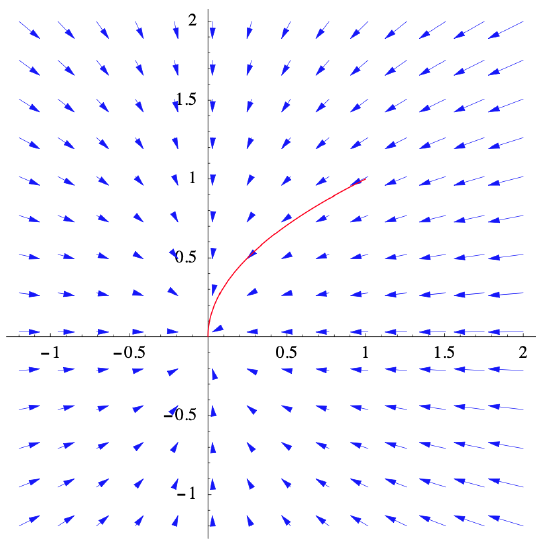
if \(C\) is the shadow of the path of the bug in the \(xy\)-plane, then the slope of \(C\) at any point \((x,y)\) would be

\[ \frac{d y}{d x}=\frac{-2 y}{-4 x}=\frac{y}{2 x} . \nonumber \]

Hence

\[ \frac{1}{y} \frac{d y}{d x}=\frac{1}{2 x} . \nonumber \]

If we integrate both sides of this equality, we have

\[\int \frac{1}{y} \frac{d y}{d x} d x=\int \frac{1}{2 x} d x . \nonumber \]

Thus

\[ \log |y|=\frac{1}{2} \log |x|+c \nonumber \]

for some constant \(c\), from which we have

\[ e^{\log |y|}=e^{\frac{1}{2} \log |x|+c} . \nonumber \]

It follows that

\[ y=k \sqrt{|x|} , \nonumber \]

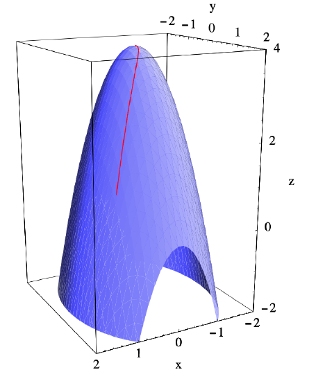
where \(k=\pm e^{c}\). Since \(y=1\) when \(x=1\), \(k=1\) and we see that \(C\) is the graph of \(y=\sqrt{x}\). Figure 3.2.2 shows \(C\) along with the plot of the gradient vectors of \(f\), while Figure 3.2.3 shows the actual path of the bug on the graph of \(f\).

Figure \(\PageIndex{3}\): Graph \(f(x, y)=4-2 x^{2}-y^{2}\) with path of most rapid ascent from (1,1,1)

Example \(\PageIndex{11}\)

For a two-dimensional version of the temperature example discussed above, consider a metal plate heated so that its temperature at \((x,y)\) is given by

\[ T(x, y)=80-20 x e^{-\frac{1}{20}\left(x^{2}+y^{2}\right)} . \nonumber \]

Then

\[ \nabla T(x, y)=e^{-\frac{1}{20}\left(x^{2}+y^{2}\right)}\left(2 x^{2}-20,2 x y\right) , \nonumber \]

so, for example,

\[ \nabla T(0,0)=(-20,0) . \nonumber \]

Thus at the origin the temperature is increasing most rapidly in the direction of \(u=(-1,0)\) and decreasing most rapidly in the direction of (1,0). Moreover,

\[ D_{\mathbf{u}} T(0,0)=\|\nabla f(0,0)\|=20 \nonumber \]

and

\[ D_{-\mathbf{u}} T(0,0)=-\|\nabla f(0,0)\|=20 . \nonumber \]

Note that

\[ D_{-\mathbf{u}} T(0,0)=\frac{\partial}{\partial x} T(0,0) \nonumber \]

and

\[ D_{\mathbf{u}} T(0,0)=-\frac{\partial}{\partial x} T(0,0) . \nonumber \]

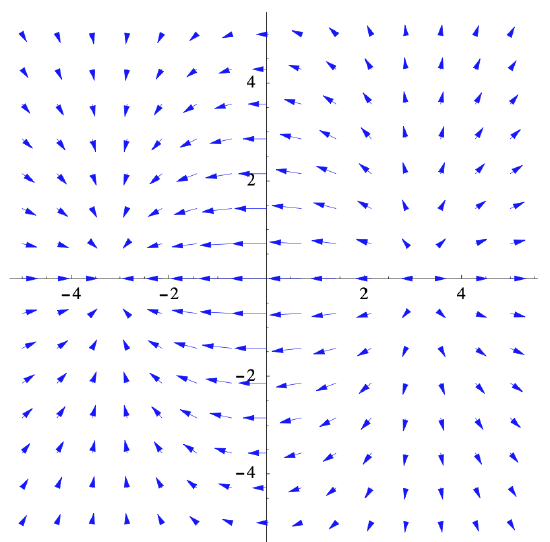
Figure 3.2.4 is a plot of scaled gradient vectors for this temperature function. From the plot it is easy to see which direction a bug placed on this metal plate would have to choose in order to warm up as rapidly as possible. It should also be clear that the temperature has a relative maximum around \((-3,0)\) and a relative minimum around \( (3,0) \); these points are, in fact, exactly \((-\sqrt{10}, 0)\) and \((\sqrt{10}, 0)\), the points where \(\nabla T(x, y)=(0,0)\). We will consider the problem of finding maximum and minimum values of functions of more than one variable in Section 3.5.

Figure \(\PageIndex{4}\): Scaled gradient vectors for \(T(x, y)=80-20 x e^{-\frac{1}{20}\left(x^{2}+y^{2}\right)}\)