3.6: Definite Integrals

We will first define the definite integral for a function \(f: \mathbb{R}^{2} \rightarrow \mathbb{R}\) and later indicate how the definition may be extended to functions of three or more variables.

Cartesian products

We will find the following notation useful. Given two sets of real numbers \(A\) and \(B\), we define the Cartesian product of \(A\) and \(B\) to be the set

\[ A \times B=\{(x, y): x \in A, y \in B\} . \]

For example, if \(A=\{1,2,3\}\) and \(B=\{5,6\}\), then

\[ A \times B=\{(1,5),(1,6),(2,5),(2,6),(3,5),(3,6)\} . \nonumber \]

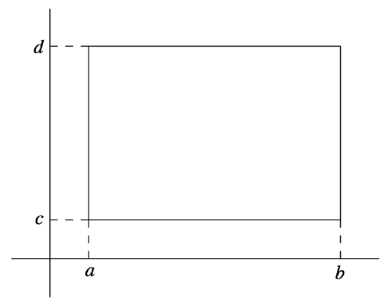
In particular, if \(a<b, c<d, A=[a, b]\), and \(B=[c, d]\), then \(A \times B=[a, b] \times[c, d]\) is the closed rectangle

\[ \{(x, y): a \leq x \leq b, c \leq y \leq d\} , \nonumber \]

as shown in Figure 3.6.1.

Figure \(\PageIndex{1}\): The closed rectangle \([a, b] \times[c, d]\)

More generally, given real numbers \(a_{i}<b_{i}, i=1,2,3, \ldots, n\), we may write

\[ \left[a_{1}, b_{1}\right] \times\left[a_{2}, b_{2}\right] \times \cdots\left[a_{n}, b_{n}\right] \nonumber \]

for the closed rectangle

\[ \left\{\left(x_{1}, x_{2}, \ldots, x_{n}\right): a_{i} \leq x_{i} \leq b_{i}, i=1,2, \ldots, n\right\} \nonumber \]

and

\[ \left(a_{1}, b_{1}\right) \times\left(a_{2}, b_{2}\right) \times \cdots\left(a_{n}, b_{n}\right) \nonumber \]

for the open rectangle

\[ \left\{\left(x_{1}, x_{2}, \ldots, x_{n}\right): a_{i}<x_{i}<b_{i}, i=1,2, \ldots, n\right\} . \nonumber \]

Definite integrals on rectangles

Given \(a<b\) and \(c<d\), let

\[ D=[a, b] \times[c, d] \nonumber \]

and suppose \(f: \mathbb{R}^{2} \rightarrow \mathbb{R}\) is defined on all of \(D\). Moreover, we suppose \(f\) is bounded on \(D\), that is, there exist constants \(m\) and \(M\) such that \(m \leq f(x, y) \leq M\) for all \((x,y)\) in \(D\). In particular, the Extreme Value Theorem implies that \(f\) is bounded on \(D\) if \(f\) is continuous on \(D\). Our definition of the definite integral of \(f\) over the rectangle \(D\) will follow the definition from one-variable calculus. Given positive integers \(m\) and \(n\), we let \(P\) be a partition of \([a,b]\) into \(m\) intervals, that is, a set \(P=\left\{x_{0}, x_{1}, \ldots, x_{m}\right\}\) where

\[ a=x_{0}<x_{1}<\cdots<x_{m}=b , \]

and we let \(Q\) be a partition of \([c,d]\) into \(n\) intervals, that is, a set \(Q=\left\{y_{0}, y_{1}, \ldots, y_{n}\right\}\) where

\[ c=y_{0}<y_{1}<\cdots<y_{n}=d . \]

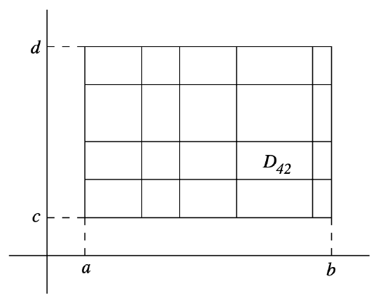
We will let \(P \times Q \) denote the partition of \(D\) into \(mn\) rectangles

\[ D_{i j}=\left[x_{i-1}, x_{i}\right] \times\left[y_{j-1}, y_{j}\right] , \]

where \(i=1,2, \ldots, m\) and \(j=1,2, \ldots, n\). Note that \(D_{i j}\) has area \(\Delta x_{i} \Delta y_{j}\), where

\[ \Delta x_{i}=x_{i}-x_{i-1} \]

and

\[ \Delta y_{j}=y_{j}-y_{j-1} . \]

An example is shown in Figure 3.6.2.

Figure \(\PageIndex{2}\): A partition of a rectangle \([a, b] \times[c, d]\)

Now let \(m_{i j}\) be the largest real number with the property that \(m_{i j} \leq f(x, y)\) for all \((x,y)\) in \(D_{ij}\) and \(M_{ij}\) be the smallest real number with the property that \(f(x, y) \leq M_{i j}\) for all \((x,y)\) in \(D_{ij}\). Note that if \(f\) is continuous on \(D\), then \(m_{ij}\) is simply the minimum value of \(f\) on \(D_{ij}\) and \(M_{ij}\) is the maximum value of \(f\) on \(D_{ij}\), both of which are guaranteed to exist by the Extreme Value Theorem. If \(f\) is not continuous, our assumption that \(f\) is bounded nevertheless guarantees the existence of the \(m_{ij}\) and \(M_{ij}\), although the justification for this statement lies beyond the scope of this book.

We may now define the lower sum, \(L(f, P \times Q)\), for \(f\) with respect to the partition \(P \times Q \) by

\[ L(f, P \times Q)=\sum_{i=1}^{m} \sum_{j=1}^{n} m_{i j} \Delta x_{i} \Delta y_{j} \]

and the upper sum, \(U(f, P \times Q)\), for \(f\) with respect to the partition \(P \times Q \) by

\[ U(f, P \times Q)=\sum_{i=1}^{m} \sum_{j=1}^{n} M_{i j} \Delta x_{i} \Delta y_{j} . \]

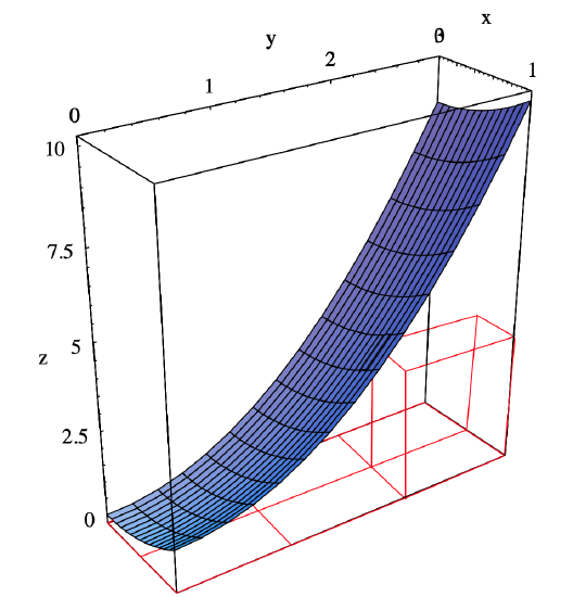
Geometrically, if \(f(x, y) \geq 0\) for all \((x,y)\) in \(D\) and \(V\) is the volume of the region which lies beneath the graph of \(f\) and above the rectangle \(D\), then \(L(f, P \times Q)\) and \(U(f, P \times Q)\) represent lower and upper bounds, respectively, for \(V\). (See Figure 3.6.3 for an example of one term of a lower sum). Moreover, we should expect that these bounds can be made arbitrarily close to \(V\) using sufficiently fine partitions \(P\) and \(Q\). In part this implies that we may characterize \(V\) as the only real number which lies between \(L(f, P \times Q)\) and \(U(f, P \times Q)\) for all choices of partitions \(P\) and \(Q\). This is the basis for the following definition.

Definition \(\PageIndex{1}\)

Suppose \(f: \mathbb{R}^{2} \rightarrow \mathbb{R}\) is bounded on the rectangle \(D=[a, b] \times[c, d]\). With the notation as above, we say \(f\) is integrable on \(D\) if there exists a unique real number \(I\) such that

\[ L(f, P \times Q) \leq I \leq U(f, P \times Q) \]

for all partitions \(P\) of \([a,b]\) and \(Q\) of \([c,d]\). If \(f\) is integrable on \(D\), we call \(I\) the definite integral of \(f\) on \(D\), which we denote

\[ I=\iint_{D} f(x, y) d x d y . \]

Geometrically, if \(f(x, y) \geq 0\) for all \((x,y)\) in \(D\), we may think of the definite integral of \(f\) on \(D\) as the volume of the region in \(R^3\) which lies beneath the graph of \(f\) and above the rectangle \(D\). Other interpretations include total mass of the rectangle \(D\) (if \(f(x,y)\) represents the density of mass at the point \((x,y)\)) and total electric charge of the rectangle \(D\) (if \(f(x,y)\) represents the charge density at the point \((x,y)\)).

Example \(\PageIndex{1}\)

Suppose \(f(x, y)=x^{2}+y^{2}\) and \(D=[0,1] \times[0,3]\). If we let

\[ P=\left\{0, \frac{1}{2}, 1\right\} \nonumber \]

and

\[ Q=\{0,1,2,3\} , \nonumber \]

then the minimum value of \(f\) on each rectangle of the partition \(P \times Q \) occurs at the lower left-hand corner of the rectangle and the maximum value of \(f\) occurs at the upper righthand corner of the rectangle. See Figure 3.6.3 for a picture of one term of the lower sum.

Figure \(\PageIndex{3}\): Graph of \(f(x, y)=x^{2}+y^{2}\) showing one term of a lower sum

Hence

\[ \begin{aligned}
L(f, P \times Q)=& f(0,0) \times \frac{1}{2} \times 1+f\left(\frac{1}{2}, 0\right) \times \frac{1}{2} \times 1+f(0,1) \times \frac{1}{2} \times 1 \\
& \quad+f\left(\frac{1}{2}, 1\right) \times \frac{1}{2} \times 1+f(0,2) \times \frac{1}{2} \times 1+f\left(\frac{1}{2}, 2\right) \times \frac{1}{2} \times 1 \\
=& 0+\frac{1}{8}+\frac{1}{2}+\frac{5}{8}+2+\frac{17}{8} \\
=& \frac{43}{8}=5.375
\end{aligned} \]

and

\[ \begin{aligned}
U(f, P \times Q)=f &\left(\frac{1}{2}, 1\right) \times \frac{1}{2} \times 1+f(1,1) \times \frac{1}{2} \times 1+f\left(\frac{1}{2}, 2\right) \times \frac{1}{2} \times 1 \\
&+f(1,2) \times \frac{1}{2} \times 1+f\left(\frac{1}{2}, 3\right) \times \frac{1}{2} \times 1+f(1,3) \times \frac{1}{2} \times 1 \\
&=\frac{5}{8}+1+\frac{17}{8}+\frac{5}{2}+\frac{37}{8}+5 \\
&=\frac{127}{8}=15.875.
\end{aligned} \]

We will see below that the continuity of \(f\) implies that \(f\) is integrable on \(D\), so we may conclude that

\[ 5.375 \leq \iint\left(x^{2}+y^{2}\right) d x d y \leq 15.875 . \nonumber \]

Example \(\PageIndex{2}\)

Suppose \(k\) is a constant and \(f(x, y)=k\) for all \((x,y)\) in the rectangle \(D=[a, b] \times[c, d]\). The for any partitions \(P=\left\{x_{0}, x_{1}, \ldots, x_{m}\right\}\) of \([a,b]\) and \(Q=\left\{y_{0}, y_{1}, \ldots, y_{n}\right\}\) of \([c,d]\), \(m_{i j}=k=M_{i j}\) for \(i=1,2, \ldots, m\) and \(j=1,2, \ldots, n\). Hence

\[ \begin{aligned}
L(f, P \times Q) &=U(f, P \times Q) \\
&=\sum_{i=1}^{m} \sum_{j=1}^{n} k \Delta x_{i} \Delta y_{j} \\
&=k \sum_{i=1}^{m} \sum_{j=1}^{n} \Delta x_{i} \Delta y_{j} \\
&=k \times(\text { area of } D) \\
&=k(b-a)(d-c).
\end{aligned} \]

Hence \(f\) is integrable and

\[ \iint_{D} f(x, y) d x d y=\iint_{D} k d x d y=k(b-a)(d-c) . \nonumber \]

Of course, geometrically this result is saying that the volume of a box with height \(k\) and base \(D\) is \(k\) times the area of \(D\). In particular, if \(k=1\) we see that

\[ \iint_{D} d x d y=\operatorname{area} \text { of } D . \nonumber \]

Example \(\PageIndex{3}\)

If \(D=[1,2] \times[-1,3]\), then

\[ \int_{D} 5 d x d y=5(2-1)(3+1)=20 . \nonumber \]

The properties of the definite integral stated in the following proposition follow easily from the definition, although we will omit the somewhat technical details.

Proposition \(\PageIndex{1}\)

Suppose \(f: \mathbb{R}^{2} \rightarrow \mathbb{R}\) and \(g: \mathbb{R}^{2} \rightarrow \mathbb{R}\) are both integrable on the rectangle \(D=[a, b] \times[c, d]\) and \(k\) is a scalar constant. Then

\[ \iint_{D}(f(x, y)+g(x, y)) d x d y=\iint_{D} f(x, y) d x d y+\iint_{D} g(x, y) d x d y ,\]

\[ \iint_{D} k f(x, y) d x d y=k \iint_{D} f(x, y) d x d y , \]

and, if \(f(x, y) \leq g(x, y)\) for all \((x,y)\) in \(D\),

\[ \iint_{D} f(x, y) d x d y \leq \iint_{D} g(x, y) d x d y . \]

Our definition does not provide a practical method for determining whether a given function is integrable or not. A complete characterization of integrability is beyond the scope of this text, but we shall find one simple condition very useful: if \(f\) is continuous on an open set containing the rectangle \(D\), then \(f\) is integrable on \(D\). Although we will not attempt a full proof of this result, the outline is as follows. If \(f\) is continuous on \(D=[a, b] \times[c, d]\) and we are given any \(\epsilon > 0\), then it is possible to find partitions \(P\) of \([a,b]\) and \(Q\) of \([c,d]\) sufficiently fine to guarantee that if \((x,y)\) and \((u,v)\) are points in the same rectangle \(D_{ij}\) of the partition \(P \times Q\) of \(D\), then

\[ |f(x, y)-f(u, v)|<\frac{\epsilon}{(b-a)(d-c)} . \]

(Note that this is not a direct consequence of the continuity of \(f\), but follows from a slightly deeper property of continuous functions on closed bounded sets known as uniform continuity.) It follows that if \(m_{ij}\) is the minimum value and \(M_{ij}\) is the maximum value of \(f\) on \(D_{ij}\), then

\[ \begin{align}
U(f, P \times Q)-L(f, P \times Q) &=\sum_{i=1}^{m} \sum_{j=1}^{n} M_{i j} \Delta x_{i} \Delta y_{j}-\sum_{i=1}^{m} \sum_{j=1}^{n} m_{i j} \Delta x_{i} \Delta y_{j} \nonumber \\
&=\sum_{i=1}^{m} \sum_{j=1}^{n}\left(M_{i j}-m_{i j}\right) \Delta x_{i} \Delta y_{j} \nonumber \\
&<\sum_{i=1}^{m} \sum_{j=1}^{n} \frac{\epsilon}{(b-a)(d-c)} \Delta x_{i} \Delta y_{j} \label{} \\
&=\frac{\epsilon}{(b-a)(d-c)} \sum_{i=1}^{m} \sum_{j=1}^{n} \Delta x_{i} \Delta y_{j} \nonumber \\
&=\frac{\epsilon}{(b-a)(d-c)}(b-a)(d-c) \nonumber \\
&=\epsilon . \nonumber
\end{align} \]

It now follows that we may find upper and lower sums which are arbitrarily close, from which follows the integrability of \(f\).

Theorem \(\PageIndex{1}\)

If \(f\) is continuous on an open set containing the rectangle \(D\), then \(f\) is integrable on \(D\).

Example \(\PageIndex{4}\)

If \(f(x, y)=x^{2}+y^{2}\), then \(f\) is continuous on all of \(R^2\). Hence \(f\) is integrable on \(D=[0,1] \times[0,3]\).

Iterated integrals

Now suppose we have a rectangle \(D=[a, b] \times[c, d]\) and a continuous function \(f: \mathbb{R}^{2} \rightarrow \mathbb{R}\) such that \(f(x, y) \geq 0\) for all \((x,y)\) in \(D\). Let

\[ B=\{(x, y, z):(x, y) \in D, 0 \leq z \leq f(x, y)\} . \]

Then \(B\) is the region in \(\mathbb{R}^3\) bounded below by \(D\) and above by the graph of \(f\). If we let \(V\) be the volume of \(B\), then

\[ V=\iint_{D} f(x, y) d x d y . \]

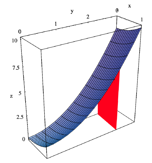
However, there is another approach to finding \(V\). If, for every \( c \leq y \leq d \), we let

\[ \alpha(y)=\int_{a}^{b} f(x, y) d x , \]

then \(\alpha(y)\) is the area of a slice of \(B\) cut by a plane orthogonal to both the \(xy\)-plane and the \(yz\)-plane and passing through the point \( (0,y,0) \) on the \(y\)-axis (see Figure 3.6.4 for an example).

Figure \(\PageIndex{4}\): A slice of the region beneath \(f(x, y)=x^{2}+y^{2}\) with area \(\alpha (2)\)

If we let the partition \(Q=\left\{y_{0}, y_{1}, \ldots, y_{n}\right\}\) divide \([c,d]\) into \(n\) intervals of equal length \(\Delta y\), then we may approximate \(V\) by

\[ \sum_{j=1}^{n} \alpha\left(y_{i}\right) \Delta y . \]

That is, we may approximate \(V\) by slicing \(B\) into slabs of thickness \(\Delta y \) perpendicular to the \(yz\)-plane, and then summing approximations to the volume of each slab. As \(n\) increases, this approximation should converge to \(V\) ; at the same time, since (3.6.19) is a right-hand rule approximation to the definite integral of \(\alpha\) over \([c,d]\), the sum should converge to

\[ \int_{c}^{d} \alpha(y) d y \nonumber \]

as \(n\) increases. That is, we should have

\[ V=\lim _{n \rightarrow \infty} \sum_{j=1}^{n} \alpha\left(y_{i}\right) \Delta y=\int_{c}^{d} \alpha(y) d y=\int_{c}^{d}\left(\int_{a}^{b} f(x, y) d x\right) d y . \label{3.6.20}\]

Note that the expression on the right-hand side of (\(\ref{3.6.20}\)) is not the definite integral of \(f\) over \(D\), but rather two successive integrals of one variable. Also, we could have reversed our order and first integrated with respect to \(y\) and then integrated the result with respect to \(x\).

Definition \(\PageIndex{2}\)

Suppose \(f: \mathbb{R}^{2} \rightarrow \mathbb{R}\) is defined on a rectangle \(D=[a, b] \times[c, d]\). The iterated integrals of \(f\) over \(D\) are

\[ \int_{c}^{d} \int_{a}^{b} f(x, y) d x d y=\int_{c}^{d}\left(\int_{a}^{b} f(x, y) d x\right) d y \label{3.6.21} \]

and

\[ \int_{a}^{b} \int_{c}^{d} f(x, y) d y d x=\int_{a}^{b}\left(\int_{c}^{d} f(x, y) d y\right) d x . \label{3.6.22} \]

In the situation of the preceding paragraph, we should expect the iterated integrals in (\(\ref{3.6.21}\)) and (\(\ref{3.6.22}\)) to be equal since they should both equal \(V\), the volume of the region \(B\). Moreover, since we also know that

\[ V=\iint_{D} f(x, y) d x d y , \nonumber \]

the iterated integrals should both be equal to the definite integral of \(f\) over \(D\). These statements may in fact be verified as long as \(f\) is integrable on \(D\) and the iterated integrals exist. In this case, iterated integrals provide a method of evaluating double integrals in terms of integrals of a single variable (for which we may use the Fundamental Theorem of Calculus).

Fubini's Theorem (for rectangles) \(\PageIndex{2}\)

Suppose \(f\) is integrable over the rectangle \(D=[a, b] \times[c, d]\). If

\[ \int_{c}^{d} \int_{a}^{b} f(x, y) d x d y \nonumber \]

exists, then

\[ \iint_{D} f(x, y) d x d y=\int_{c}^{d} \int_{a}^{b} f(x, y) d x d y . \]

If

\[ \int_{a}^{b} \int_{c}^{d} f(x, y) d y d x \nonumber \]

exists, then

\[ \iint_{D} f(x, y) d x d y=\int_{a}^{b} \int_{c}^{d} f(x, y) d x d y . \]

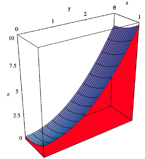
Example \(\PageIndex{5}\)

To find the volume \(V\) of the region beneath the graph of \(f(x, y)=x^{2}+y^{2}\) and over the rectangle \(D=[0,1] \times[0,3]\) (as shown in Figure 3.6.5), we compute

\[ \begin{aligned}
V &=\iint_{D}\left(x^{2}+y^{2}\right) d x d y \\
&=\int_{0}^{3} \int_{0}^{1}\left(x^{2}+y^{2}\right) d x d y
\end{aligned} \]

\[ \begin{aligned}
&=\left.\int_{0}^{3}\left(\frac{x^{3}}{3}+x y^{2}\right)\right|_{0} ^{1} d y \\
&=\int_{0}^{3}\left(\frac{1}{3}+y^{2}\right) d y \\
&=\left.\left(\frac{y}{3}+\frac{y^{3}}{3}\right)\right|_{0} ^{3} \\
&=1+9 \\
&=10 .
\end{aligned} \]

Figure \(\PageIndex{5}\): Region beneath \(f(x, y)=x^{2}+y^{2}\) over the rectangle \([0,1] \times[0,3]\)

We could also compute the iterated integral in the other order:

\[ \begin{aligned}
V &=\iint_{D}\left(x^{2}+y^{2}\right) d x d y \\
&=\int_{0}^{1} \int_{0}^{3}\left(x^{2}+y^{2}\right) d y d x \\
&=\left.\int_{0}^{1}\left(x^{2} y+\frac{y^{3}}{3}\right)\right|_{0} ^{3} d x \\
&=\int_{0}^{1}\left(3 x^{2}+9\right) d x \\
&=\left.\left(x^{3}+9 y\right)\right|_{0} ^{1} \\
&=1+9 \\
&=10.
\end{aligned} \]

Example \(\PageIndex{6}\)

If \(D=[1,2] \times[0,1]\), then

\[ \iint_{D} x^{2} y d x d y=\int_{1}^{2} \int_{0}^{1} x^{2} y d y d x=\left.\int_{1}^{2} \frac{x^{2} y^{2}}{2}\right|_{0} ^{1} d x=\int_{1}^{2} \frac{x^{2}}{2} d x=\left.\frac{x^{3}}{6}\right|_{1} ^{2}=\frac{8}{6}-\frac{1}{6}=\frac{7}{6} . \nonumber \]

Definite integrals on other regions

Integrals over intervals suffice for most applications of functions of a single variable. However, for functions of two variables it is important to consider integrals on regions other than rectangles. To extend our definition, consider a function \(f: \mathbb{R}^{2} \rightarrow \mathbb{R}\) defined on a bounded region \(D\). Let \(D^{*}\) be a rectangle containing \(D\) and, for any \((x,y)\) in \(D^{*}\), define

\[ f^{*}(x, y)= \begin{cases}f(x, y), & \text { if }(x, y) \in D, \\ 0, & \text { if }(x, y) \notin D. \end{cases} \label{3.6.25} \]

In other words, \(f^*\) is identical to \(f\) on \(D\) and 0 at all points of \(D^*\) outside of \(D\). Now if \(f^*\) is integrable on \(D^*\), and since the the region where \(f^*\) is 0 should contribute nothing to the value of the integral, it is reasonable to define the integral of \(f\) over \(D\) to be equal to the integral of \(f^*\) over \(D^*\).

Definition \(\PageIndex{3}\)

Suppose \(f\) is defined on a bounded region \(D\) of \(\mathbb{R}^2\) and let \(D^*\) be any rectangle containing \(D\). Define \(f^*\) as in (\(\ref{3.6.25}\)). We say \(f\) is integrable on \(D\) if \(f^*\) is integrable on \(D^*\), in which case we define

\[ \iint_{D} f(x, y) d x d y=\iint_{D^{*}} f^{*}(x, y) d x d y . \]

Note that the integrability of \(f\) on a region \(D\) depends not only on the nature of \(f\), but on the region \(D\) as well. In particular, even if \(f\) is continuous on an open set containing \(D\), it may still turn out that \(f\) is not integrable on \(D\) because of the complicated nature of the boundary of \(D\). Fortunately, there are two basic types of regions which occur frequently and to which our previous theorems generalize.

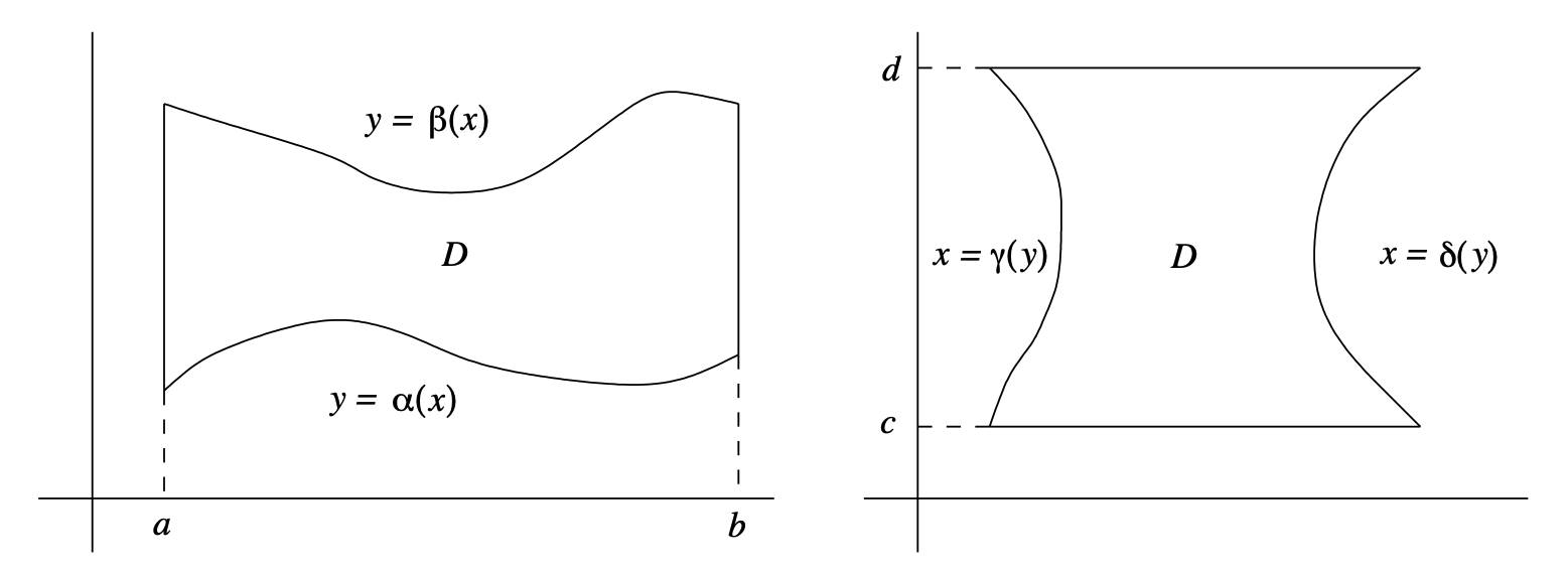
Definition \(\PageIndex{4}\)

We say a region \(D\) in \(\mathbb{R}^2\) is of Type I if there exist real numbers \(a<b\) and continuous functions \(\alpha: \mathbb{R} \rightarrow \mathbb{R}\) and \(\beta: \mathbb{R} \rightarrow \mathbb{R}\) such that \(\alpha(x) \leq \beta(x)\) for all \(x\) in \([a,b]\) and

\[ D=\{(x, y): a \leq x \leq b, \alpha(x) \leq y \leq \beta(x)\} . \]

We say a region \(D\) in \(R^2\) is of Type II if there exist real numbers \(c<d\) and continuous functions \(\gamma: \mathbb{R} \rightarrow \mathbb{R}\) and \(\delta: \mathbb{R} \rightarrow \mathbb{R}\) such that \(\gamma(y) \leq \delta(y)\) for all \(y\) in \([c,d]\) and

\[ D=\{(x, y): c \leq y \leq d, \gamma(y) \leq x \leq \delta(y)\} . \]

Figure 3.6.6 shows typical examples of regions of Type I and Type II.

Figure \(\PageIndex{6}\): Regions of Type I and Type II

Example \(\PageIndex{7}\)

If \(D\) is the triangle with vertices at (0,0), (1,0), and (1,1), then

\[ D=\{(x, y): 0 \leq x \leq 1,0 \leq y \leq x\} . \nonumber \]

Hence \(D\) is a Type I region with \(\alpha(x)=0\) and \(\beta(x)=x .\) Note that we also have

\[ D=\{(x, y): 0 \leq y \leq 1, y \leq x \leq 1\} , \nonumber \]

so \(D\) is also a Type II region with \(\gamma(y)=y\) and \(\delta(y)=1\). See Figure 3.6.7.

Figure \(\PageIndex{7}\): Two regions which are of both Type I and Type II

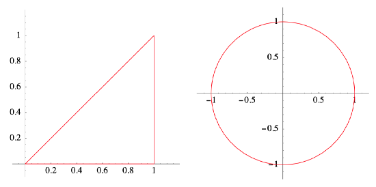
Example \(\PageIndex{8}\)

The closed disk

\[ D=\left\{(x, y): x^{2}+y^{2} \leq 1\right\} \nonumber \]

is both a region of Type I, with

\[ D=\left\{(x, y):-1 \leq x \leq 1,-\sqrt{1-x^{2}} \leq y \leq \sqrt{1-x^{2}}\right\} , \nonumber \]

and a region of Type II, with

\[ D=\left\{(x, y):-1 \leq y \leq 1,-\sqrt{1-y^{2}} \leq x \leq \sqrt{1-x^{2}}\right\} . \nonumber \]

See Figure 3.6.7.

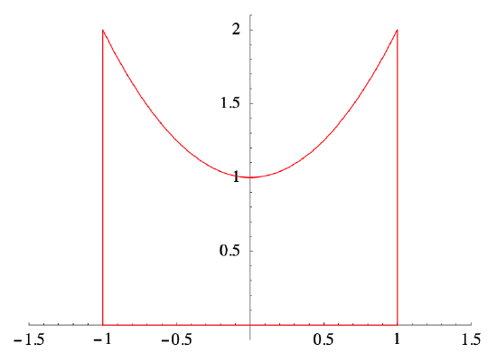
Example \(\PageIndex{9}\)

Let \(D\) be the region which lies beneath the graph of \(y=x^2\) and above the interval \( [−1,1] \) on the \(x\)-axis. Then

\[ D=\left\{(x, y):-1 \leq x \leq 1,0 \leq y \leq x^{2}\right\} , \nonumber \]

so \(D\) is a region of Type I. However, \(D\) is not a region of Type II. See Figure 3.6.8.

Figure \(\PageIndex{8}\): A region which is of Type I but not of Type II

Theorem \(\PageIndex{3}\)

If \(D\) is a region of Type I or a region of Type II and \(f: \mathbb{R}^{2} \rightarrow \mathbb{R}\) is continuous on an open set containing \(D\), then \(f\) is integrable on \(D\).

Fubini's Theorem (for regions of Type I and Type II) \(\PageIndex{4}\)

Suppose \(f: \mathbb{R}^{2} \rightarrow \mathbb{R}\) is integrable on the region \(D\). If \(D\) is a region of Type I with

\[ D=\{(x, y): a \leq x \leq b, \alpha(x) \leq y \leq \beta(x)\} \nonumber \]

and the iterated integral

\[ \int_{a}^{b} \int_{\alpha(x)}^{\beta(x)} f(x, y) d y d x \nonumber \]

exists, then

\[ \iint_{D} f(x, y) d x d y=\int_{a}^{b} \int_{\alpha(x)}^{\beta(x)} f(x, y) d y d x . \]

If \(D\) is a region of Type II with

\[ D=\{(x, y): c \leq y \leq d, \gamma(y) \leq x \leq \delta(y)\} \nonumber \]

and the iterated integral

\[ \int_{c}^{d} \int_{\gamma(y)}^{\delta(y)} f(x, y) d x d y \nonumber \]

exists, then

\[ \iint_{D} f(x, y) d x d y=\int_{c}^{d} \int_{\gamma(y)}^{\delta(y)} f(x, y) d y d x . \]

Example \(\PageIndex{10}\)

Let \(D\) be the triangle with vertices at (0,0), (1,0), and (1,1), as in the example above. Expressing \(D\) as a region of Type I, we have

\[ \iint_{D} x y d x d y=\int_{0}^{1} \int_{0}^{x} x y d y d x=\left.\int_{0}^{1} \frac{x y^{2}}{2}\right|_{0} ^{x} d x=\int_{0}^{1} \frac{x^{3}}{2} d x=\left.\frac{x^{4}}{8}\right|_{0} ^{1}=\frac{1}{8} . \nonumber \]

Since \(D\) is also a region of Type II, we may evaluate the integral in the other order as well, obtaining

\[ \iint_{D} x y d x d y=\int_{0}^{1} \int_{y}^{1} x y d x d y=\left.\int_{0}^{1} \frac{x^{2} y}{2}\right|_{y} ^{1} d y=\int_{0}^{1}\left(\frac{y}{2}-\frac{y^{3}}{2}\right) d y=\left.\left(\frac{y^{2}}{4}-\frac{y^{4}}{8}\right)\right|_{0} ^{1}=\frac{1}{8} . \nonumber \]

In the last example the choice of integration was not too important, with the first order being perhaps slightly easier than the second. However, there are times when the choice of the order of integration has a significant effect on the ease of integration.

Example \(\PageIndex{11}\)

Let \(D=\{(x, y): 0 \leq x \leq 1, \sqrt{x} \leq y \leq 1\}\) (see Figure 3.6.9).

Figure \(\PageIndex{9}\): The region \(D=\{(x, y): 0 \leq x \leq 1, \sqrt{x} \leq y \leq 1\}\)

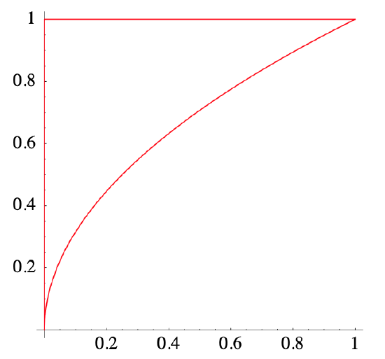
Since \(D\) is both of Type I and of Type II, we may evaluate

\[ \iint_{D} e^{-y^{3}} d x d y \nonumber \]

either as

\[ \int_{0}^{1} \int_{\sqrt{x}}^{1} e^{-y^{3}} d y d x \nonumber \]

or as

\[ \int_{0}^{1} \int_{0}^{y^{2}} e^{-y^{3}} d x d y . \nonumber \]

The first of these two iterated integrals requires integrating \(g(y)=e^{-y^{3}}\); however, we may evaluate the second easily:

\[ \begin{aligned}
\iint_{D} e^{-y^{3}} d x d y &=\int_{0}^{1} \int_{0}^{y^{2}} e^{-y^{3}} d x d y \\
&=\left.\int_{0}^{1} x e^{-y^{3}}\right|_{0} ^{y^{2}} d y \\
&=\int_{0}^{1} y^{2} e^{-y^{3}} d y \\
&=-\left.\frac{1}{3} e^{-y^{3}}\right|_{0} ^{1} \\
&=\frac{1}{3}\left(1-e^{-1}\right).
\end{aligned} \]

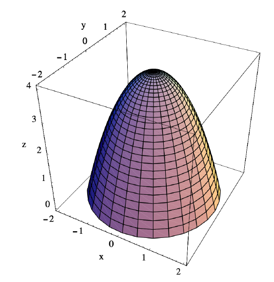
Example \(\PageIndex{12}\)

Let \(V\) be the volume of the region lying below the paraboloid \(P\) with equation \(z=4-x^{2}-y^{2}\) and above the \(xy\)-plane (see Figure 3.6.10).

Figure \(\PageIndex{10}\): Region bounded by \(z=4-x^{2}-y^{2}\) and the \(xy\)-plane

Since the surface \(P\) intersects the \(xy\)-plane when

\[ 4-x^{2}-y^{2}=0 , \nonumber \]

that is, when

\[ x^{2}+y^{2}=4 , \nonumber \]

\(V\) is the volume of the region bounded above by the graph of \(f(x, y)=4-x^{2}-y^{2}\) and below by the region

\[ D=\left\{(x, y): x^{2}+y^{2} \leq 4\right\} . \nonumber \]

If we describe \(D\) as a Type I region, namely,

\[ D=\left\{(x, y):-2 \leq x \leq 2,-\sqrt{4-x^{2}} \leq y \leq \sqrt{4-x^{2}}\right\} , \nonumber \]

then we may compute

\[ \begin{aligned}
V &=\iint_{D}\left(4-x^{2}-y^{2}\right) d x d y \\
&=\int_{-2}^{2} \int_{-\sqrt{4-x^{2}}}^{\sqrt{4-x^{2}}}\left(4-x^{2}-y^{2}\right) d y d x \\
&=\left.\int_{-2}^{2}\left(4 y-x^{2} y-\frac{y^{3}}{3}\right)\right|_{-\sqrt{4-x^{2}}} ^{\sqrt{4-x^{2}}} d x \\
&=\int_{-2}^{2}\left(8 \sqrt{4-x^{2}}-2 x^{2} \sqrt{4-x^{2}}-\frac{2}{3}\left(4-x^{2}\right)^{\frac{3}{2}}\right) d x \\
&=2 \int_{-2}^{2}\left(\left(4-x^{2}\right) \sqrt{4-x^{2}}-\frac{1}{3}\left(4-x^{2}\right)^{\frac{3}{2}}\right) d x \\
&=\frac{4}{3} \int_{-2}^{2}\left(4-x^{2}\right)^{\frac{3}{2}} d x.
\end{aligned}\]

Using the substitution \(x=2 \sin (\theta)\), we have \(d x=2 \cos (\theta) d \theta\), and so

\[ \begin{aligned}
V &=\frac{4}{3} \int_{-2}^{2}\left(4-x^{2}\right)^{\frac{3}{2}} d x \\
&=\frac{4}{3} \int_{-\frac{\pi}{2}}^{\frac{\pi}{2}}\left(4-4 \sin ^{2}(\theta)\right)^{\frac{3}{2}} 2 \cos (\theta) d \theta \\
&=\frac{64}{3} \int_{-\frac{\pi}{2}}^{\frac{\pi}{2}} \cos ^{4}(\theta) d \theta \\
&=\frac{64}{3} \int_{-\frac{\pi}{2}}^{\frac{\pi}{2}}\left(\frac{1+\cos (2 \theta)}{2}\right)^{2} d \theta \\
&=\frac{16}{3} \int_{-\frac{\pi}{2}}^{\frac{\pi}{2}}\left(1+2 \cos (2 \theta)+\cos ^{2}(2 \theta)\right) d \theta \\
&=\frac{16}{3}\left(\left.\theta\right|_{-\frac{\pi}{2}} ^{\frac{\pi}{2}}+\left.\sin (2 \theta)\right|_{-\frac{\pi}{2}} ^{\frac{\pi}{2}}+\int_{-\frac{\pi}{2}}^{\frac{\pi}{2}} \frac{1+\cos (4 \theta)}{2} d \theta\right) \\
&=\frac{16}{3}\left(\pi+\left.\frac{\theta}{2}\right|_{-\frac{\pi}{2}} ^{\frac{\pi}{2}}+\left.\frac{1}{8} \sin (4 \theta)\right|_{-\frac{\pi}{2}} ^{\frac{\pi}{2}}\right) \\
&=\frac{16}{3}\left(\pi+\frac{\pi}{2}\right) \\
&=8 \pi .
\end{aligned} \]

Integrals of functions of three or more variables

We will now sketch how to extend the definition of the definite integral to higher dimensions. Suppose \(f: \mathbb{R}^{n} \rightarrow \mathbb{R}\) is bounded on an \(n\)-dimensional closed rectangle

\[ D=\left[a_{1}, b_{1}\right] \times\left[a_{2}, b_{2}\right] \times \cdots\left[a_{n}, b_{n}\right] . \nonumber \]

Let \(P_{1}, P_{2}, \ldots, P_{n}\) partition the intervals \(\left[a_{1}, b_{1}\right],\left[a_{2}, b_{2}\right], \ldots,\left[a_{n}, b_{n}\right]\) into \(m_{1}, m_{2}, \ldots , m_n \), respectively, intervals, and let \(P_{1} \times P_{2} \times \cdots \times P_{n}\) represent the corresponding partition of \(D\) into \(m_{1} m_{2} \cdots m_{n}\) \(n\)-dimensional closed rectangles \(D_{i_{1} i_{2} \cdots i_{n}}\). If \(m_{i_{1} i_{2} \cdots i_{n}}\) is the largest real number such that \(m_{i_{1} i_{2} \cdots i_{n}} \leq f(\mathbf{x})\) for all \(\mathbf{x}\) in \(D_{i_{1} i_{2} \cdots i_{n}}\) and \(M_{i_{1} i_{2} \cdots i_{n}}\) is the smallest real number such that \(f(\mathbf{x}) \leq M_{i_{1} i_{2} \cdots i_{n}}\) for all \(\mathbf{x}\) in \(D_{i_{1} i_{2} \cdots i_{n}}\), then we may define the lower sum

\[ L\left(f, P_{1} \times P_{2} \times \cdots \times P_{n}\right)=\sum_{i_{1}=1}^{m_{1}} \sum_{i_{2}}^{m_{2}} \cdots \sum_{i_{n}=1}^{m_{n}} m_{i_{1} i_{2} \cdots i_{n}} \Delta x_{1 i_{1}} \Delta x_{2 i_{2}} \cdots \Delta x_{n i_{n}} \]

and the upper sum

\[ U\left(f, P_{1} \times P_{2} \times \cdots \times P_{n}\right)=\sum_{i_{1}=1}^{m_{1}} \sum_{i_{2}}^{m_{2}} \cdots \sum_{i_{n}=1}^{m_{n}} M_{i_{1} i_{2} \cdots i_{n}} \Delta x_{1 i_{1}} \Delta x_{2 i_{2}} \cdots \Delta x_{n i_{n}} , \]

where \(\Delta x_{j k}\) is the length of the \(k\)th interval of the partition \(P_j\). We then say \(f\) is integrable on \(D\) if there exists a unique real number \(I\) with the property that

\[ L\left(f, P_{1} \times P_{2} \times \cdots \times P_{n}\right) \leq I \leq U\left(f, P_{1} \times P_{2} \times \cdots \times P_{n}\right) \]

for all choices of partitions \(P_{1}, P_{2}, \ldots, P_{n}\) and we write

\[ I=\int \cdots \iint_{D} f\left(x_{1}, x_{2}, \ldots, x_{n}\right) d x_{1} d x_{2} \cdots d x_{n} , \]

or

\[ I=\int \cdots \iint_{D} f(\mathbf{x}) d \mathbf{x} , \]

for the definite integral of \(f\) on \(D\).

We may now generalize the definition of the integral to more general regions in the same manner as above. Moreover, our integrability theorem and Fubini’s theorem, with appropriate changes, hold as well. When \(n=3\), we may interpret

\[ \iiint_{D} f(x, y, z) d x d y d z \]

to be the total mass of \(D\) if \(f(x,y,z)\) represents the density of mass at \((x,y,z)\), or the total electric charge of \(D\) if \(f(x,y,z)\) represents the electric charge density at \((x,y,z)\). For any value of \(n\) we may interpret

\[ \int \cdots \iint_{D} d x_{1} d x_{2} \cdots d x_{n} \]

to be the \(n\)-dimensional volume of \(D\). We will not go into further details, preferring to illustrate with examples.

Example \(\PageIndex{13}\)

Suppose \(D\) is the closed rectangle

\[ \begin{aligned}
D &=\{(x, y, z, t): 0 \leq x \leq 1,-1 \leq y \leq 1,-2 \leq z \leq 2,0 \leq t \leq 2\} \\
&=[0,1] \times[-1,1] \times[-2,2] \times[0,2] .
\end{aligned} \]

Then

\[ \begin{aligned}
\iiint \int_{D}\left(x^{2}+y^{2}+z^{2}-t^{2}\right) d x d y d z d t &=\int_{0}^{1} \int_{-1}^{1} \int_{-2}^{2} \int_{0}^{2}\left(x^{2}+y^{2}+z^{2}-t^{2}\right) d t d z d y d x \\
&=\left.\int_{0}^{1} \int_{-1}^{1} \int_{-2}^{2}\left(x^{2} t+y^{2} t+z^{2} t-\frac{t^{3}}{3}\right)\right|_{0} ^{2} d z d y d x \\
&=\int_{0}^{1} \int_{-1}^{1} \int_{-2}^{2}\left(2 x^{2}+2 y^{2}+2 z^{2}-\frac{8}{3}\right) d z d x d y \\
&=\left.\int_{0}^{1} \int_{-1}^{1}\left(2 x^{2} z+2 y^{2} z+\frac{2 z^{3}}{3}-\frac{8 z}{3}\right)\right|_{-2} ^{2} d y d x \\
&=\int_{0}^{1} \int_{-1}^{1}\left(8 x^{2}+8 y^{2}+\frac{32}{3}-\frac{32}{3}\right) d y d x \\
&=\left.\int_{0}^{1}\left(8 x^{2} y+\frac{8 y^{2}}{3}\right)\right|_{-1} ^{1} d x \\
&=\int_{0}^{1}\left(16 x^{2}+\frac{16}{3}\right) d x \\
&=\left.\left(\frac{16 x^{3}}{3}+\frac{16 x}{3}\right)\right|_{0} ^{1} \\
&=\frac{32}{3}.
\end{aligned} \]

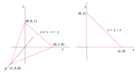
Example \(\PageIndex{14}\)

Let \(D\) be the region in \(\mathbb{R}^3\) bounded by the the three coordinate planes and the plane \(P\) with equation \(z=1-x-y\) (see Figure 3.6.11).

Figure \(\PageIndex{11}\): Region bounded by the coordinate planes and the plane \(z=1-x-y\)

Suppose we wish to evaluate

\[ \iiint_{D} x y z d x d y d z . \nonumber \]

Note that the side of \(D\) which lies in the \(xy\)-plane, that is, the plane \(z=0\), is a triangle with vertices at (0,0,0), (1,0,0), and (0,1,0). Or, strictly in terms of \(x\) and \(y\) coordinates, we may describe this face as the triangle in the first quadrant bounded by the line \(y=1-x\) (see Figure 3.6.11). Hence \(x\) varies from 0 to 1, and, for each value of \(x\), \(y\) varies from 0 to \(1-x\). Finally, once we have fixed a values for \(x\) and \(y\), \(z\) varies from 0 up to \(P\), that is, to \(1-x-y\). Hence we have

\[ \begin{aligned}
\iiint_{D} x y z d x d y d z &=\int_{0}^{1} \int_{0}^{1-x} \int_{0}^{1-x-y} x y z d z d y d x \\
&=\left.\int_{0}^{1} \int_{0}^{1-x} \frac{x y z^{2}}{2}\right|_{0} ^{1-x-y} d y d x \\
&=\int_{0}^{1} \int_{0}^{1-x} \frac{x y(1-x-y)^{2}}{2} d y d x \\
&=\frac{1}{2} \int_{0}^{1} \int_{0}^{1-x}\left(x y-2 x^{2} y+x^{3} y+2 x^{2} y^{2}+x y^{3}\right) d y d x \\
&=\left.\frac{1}{2} \int_{0}^{1}\left(\frac{x y^{2}}{2}-2 x^{2} y^{2}+\frac{x^{3} y^{2}}{2}+\frac{2 x^{2} y^{3}}{3}+\frac{x y^{4}}{4}\right)\right|_{0} ^{1-x} d x \\
&=\frac{1}{2} \int_{0}^{1}\left(\frac{3 x}{4}-\frac{10 x^{2}}{3}+\frac{9 x^{3}}{2}-2 x^{4}+\frac{x^{5}}{12}\right) d x \\
&=\left.\frac{1}{2} \int_{0}^{1}\left(\frac{3 x^{2}}{8}-\frac{10 x^{3}}{9}+\frac{9 x^{4}}{8}-\frac{2 x^{5}}{5}+\frac{x^{6}}{72}\right)\right|_{0} ^{1} \\
&=\frac{1}{2}\left(\frac{3}{8}-\frac{10}{9}+\frac{9}{8}-\frac{2}{5}+\frac{1}{72}\right) \\
&=\frac{1}{720}.
\end{aligned} \]

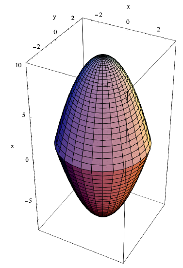
Example \(\PageIndex{15}\)

Let \(V\) be the volume of the region \(D\) in \(\mathbb{R}^3\) bounded by the paraboloids with equations \(z=10-x^{2}-y^{2}\) and \(z=x^{2}+y^{2}-8\) (see Figure 3.6.12).

Figure \(\PageIndex{12}\): Region bounded by \(z=10-x^{2}-y^{2}\) and \(z=x^{2}+y^{2}-8\)

We will find \(V\) by evaluating

\[ V=\iiint_{D} d x d y d z . \nonumber \]

To set up an iterated integral, we first note that the paraboloid \(z=10-x^{2}-y^{2}\) opens downward about the \(z\)-axis and the paraboloid \(z=x^{2}+y^{2}-8\) opens upward about the \(z\) axis. The two paraboloids intersect when

\[ 10-x^{2}-y^{2}=x^{2}+y^{2}-8 , \nonumber \]

that is, when

\[ x^{2}+y^{2}=9 . \nonumber \]

Now we may describe the region in the \(xy\)-plane described by \(x^2 + y^2 \leq 9 \) as the set of points \((x,y)\) for which \(-3 \leq x \leq 3 \) and, for every such fixed \(x\),

\[ -\sqrt{3-x^{2}} \leq y \leq \sqrt{3-x^{2}} . \nonumber \]

Moreover, once we have fixed \(x\) and \(y\) so that \((x,y)\) is inside the circle \(x^2 + y^2 = 9 \), then \((x,y,z)\) is in \(D\) provided \(x^{2}+y^{2}-8 \leq z \leq 10-x^{2}-y^{2}\). Hence we have

\[ \begin{aligned}
V &=\iiint_{D} d x d y d z \\
&=\int_{-3}^{3} \int_{-\sqrt{9-x^{2}}}^{\sqrt{9-x^{2}}} \int_{x^{2}+y^{2}-8}^{10-x^{2}-y^{2}} d z d y d x \\
&=\left.\int_{-3}^{3} \int_{-\sqrt{9-x^{2}}}^{\sqrt{9-x^{2}}} z\right|_{x^{2}+y^{2}-8} ^{10-x^{2}-y^{2}} d y d x \\
&=\int_{-3}^{3} \int_{-\sqrt{9-x^{2}}}^{\sqrt{9-x^{2}}}\left(18-2 x^{2}-2 y^{2}\right) d y d x \\
&=\left.\int_{-3}^{3}\left(18 y-2 x^{2} y-\frac{2 y^{3}}{3}\right)\right|_{-\sqrt{9-x^{2}}} ^{\sqrt{9-x^{2}}} d x \\
&=\int_{-3}^{3}\left(36 \sqrt{9-x^{2}}-4 x^{2} \sqrt{9-x^{2}}-\frac{4}{3}\left(9-x^{2}\right)^{\frac{3}{2}}\right) d x \\
&=\int_{-3}^{3} \sqrt{9-x^{2}}\left(36-4 x^{2}-\frac{4}{3}\left(9-x^{2}\right)\right) d x \\
&=\frac{8}{3} \int_{-3}^{3}\left(9-x^{2}\right)^{\frac{3}{2}} d x.
\end{aligned} \]

Using the substitution \(x=3 \sin (\theta)\), we have \(d x=3 \cos (\theta) d \theta\), and so

\[ \begin{aligned}
V &=\frac{8}{3} \int_{-3}^{3}\left(9-x^{2}\right)^{\frac{3}{2}} d x \\
&=\frac{8}{3} \int_{-\frac{\pi}{2}}^{\frac{\pi}{2}}\left(9-9 \sin ^{2}(x)\right)^{\frac{3}{2}}(3 \cos (\theta)) d \theta \\
&=216 \int_{-\frac{\pi}{2}}^{\frac{\pi}{2}} \cos ^{4}(\theta) d \theta \\
&=216 \int_{-\frac{\pi}{2}}^{\frac{\pi}{2}}\left(\frac{1+\cos (2 \theta)}{2}\right)^{2} d \theta \\
&=54 \int_{-\frac{\pi}{2}}^{\frac{\pi}{2}}\left(1+2 \cos (2 \theta)+\cos ^{2}(2 \theta)\right) d \theta \\
&=54\left(\left.\theta\right|_{-\frac{\pi}{2}} ^{\frac{\pi}{2}}+\left.\sin (2 \theta)\right|_{-\frac{\pi}{2}} ^{\frac{\pi}{2}}+\int_{-\frac{\pi}{2}}^{\frac{\pi}{2}} \frac{1+\cos (4 \theta)}{2} d \theta\right) \\
&=54 \pi+\left.27 \theta\right|_{-\frac{\pi}{2}} ^{\frac{\pi}{2}}+\left.\frac{27}{4} \sin (4 \theta)\right|_{-\frac{\pi}{2}} ^{\frac{\pi}{2}} \\
&=81 \pi .
\end{aligned} \]