4.6: Gradient, Divergence, Curl, and Laplacian

In this final section we will establish some relationships between the gradient, divergence and curl, and we will also introduce a new quantity called the Laplacian. We will then show how to write these quantities in cylindrical and spherical coordinates.

Gradient

For a real-valued function $f (x, y, z)$ on $\mathbb{R}^ 3$, the gradient $∇f (x, y, z)$ is a vector-valued function on $\mathbb{R}^ 3$, that is, its value at a point $(x, y, z)$ is the vector

$$\nonumber ∇f (x, y, z) = \left ( \dfrac{∂f}{ ∂x} , \dfrac{∂f}{ ∂y} , \dfrac{∂f}{ ∂z} \right ) = \dfrac{∂f}{ ∂x}\textbf{i} + \dfrac{∂f}{ ∂y}\textbf{j} + \dfrac{∂f}{ ∂z}\textbf{k}$$

in $\mathbb{R}^ 3$, where each of the partial derivatives is evaluated at the point $(x, y, z)$. So in this way, you can think of the symbol $∇$ as being “applied” to a real-valued function $f$ to produce a vector $∇f$.

It turns out that the divergence and curl can also be expressed in terms of the symbol $∇$. This is done by thinking of $∇$ as a vector in $\mathbb{R}^ 3$, namely

$$∇ = \dfrac{∂}{ ∂x}\textbf{i} + \dfrac{∂}{ ∂y}\textbf{j} + \dfrac{∂}{ ∂z}\textbf{k} .\label{Eq4.51}$$

Here, the symbols $\dfrac{∂}{ ∂x} ,\, \dfrac{∂}{∂y} \text{ and }\dfrac{∂}{ ∂z}$ are to be thought of as “partial derivative operators” that will get “applied” to a real-valued function, say $f (x, y, z)$, to produce the partial derivatives $\dfrac{∂f}{ ∂x} ,\, \dfrac{ ∂f}{ ∂y}\text{ and }\dfrac{∂f}{ ∂z}$. For instance, $\dfrac{∂}{ ∂x}$ “applied” to $f (x, y, z) \text{ produces }\dfrac{∂f}{ ∂x}$.

Is $∇$ really a vector? Strictly speaking, no, since $\dfrac{∂}{ ∂x} ,\, \dfrac{∂}{ ∂y} \text{ and }\dfrac{∂}{ ∂z}$ are not actual numbers. But it helps to think of $∇$ as a vector, especially with the divergence and curl, as we will soon see. The process of “applying” $\dfrac{∂}{ ∂x} ,\, \dfrac{∂}{ ∂y} ,\, \dfrac{∂}{ ∂z}$ to a real-valued function $f (x, y, z)$ is normally thought of as multiplying the quantities:

$$\nonumber \left ( \dfrac{∂}{ ∂x} \right ) (f ) = \dfrac{∂f}{ ∂x},\, \left ( \dfrac{∂}{ ∂y} \right ) (f ) = \dfrac{∂f}{ ∂y} ,\, \left ( \dfrac{∂}{ ∂z} \right ) (f ) = \dfrac{∂f}{ ∂z}$$

For this reason, $∇$ is often referred to as the “del operator”, since it “operates” on functions.

Divergence

For example, it is often convenient to write the divergence div f as $∇ \cdot \textbf{f}$, since for a vector field $\textbf{f}(x, y, z) = f_1(x, y, z)\textbf{i}+ f_2(x, y, z)\textbf{j}+ f_3(x, y, z)\textbf{k}$, the dot product of f with $∇$ (thought of as a vector) makes sense:

$$\nonumber \begin{align} ∇·\textbf{f} &= \left ( \dfrac{∂}{ ∂x}\textbf{i} + \dfrac{∂}{ ∂y}\textbf{j} + \dfrac{∂}{ ∂z}\textbf{k} \right ) · (f_1(x, y, z)\textbf{i} + f_2(x, y, z)\textbf{j} + f_3(x, y, z)\textbf{k}) \\[4pt] \nonumber &= \left ( \dfrac{∂}{ ∂x} \right ) (f_1) + \left ( \dfrac{∂}{ ∂y} \right ) (f_2) + \left ( \dfrac{∂}{ ∂z} \right ) (f_3) \\[4pt] \nonumber &= \dfrac{∂f_1}{ ∂x} + \dfrac{∂f_2}{ ∂y} + \dfrac{∂f_3}{ ∂z} \\[4pt] \nonumber &= \text{div }\textbf{f} \\[4pt] \end{align}$$

We can also write curl f in terms of $∇$, namely as $∇ × \textbf{f}$, since for a vector field $\textbf{f}(x, y, z) = P(x, y, z)\textbf{i}+Q(x, y, z)\textbf{j}+ R(x, y, z)\textbf{k}$, we have:

$$\nonumber \begin{align} ∇ × \textbf{f} &= \begin{vmatrix} \textbf{i} & \textbf{j} & \textbf{k} \\[4pt] \dfrac{∂}{ ∂x} & \dfrac{∂}{ ∂y} & \dfrac{∂}{ ∂z} \\[4pt] \nonumber P(x, y, z) & Q(x, y, z) & R(x, y, z) \\[4pt] \end{vmatrix} \\[4pt] \nonumber &=\left ( \dfrac{∂R}{ ∂y} − \dfrac{∂Q}{ ∂z}\right )\textbf{i} − \left ( \dfrac{∂R}{ ∂x} − \dfrac{∂P}{ ∂z} \right )\textbf{j} + \left ( \dfrac{∂Q}{ ∂x} − \dfrac{∂P}{ ∂y} \right )\textbf{k} \\[4pt] \nonumber &= \left ( \dfrac{∂R}{ ∂y} − \dfrac{∂Q}{ ∂z}\right )\textbf{i} + \left (\dfrac{∂P}{ ∂z}-\dfrac{∂R}{ ∂x} \right )\textbf{j} + \left ( \dfrac{∂Q}{ ∂x} − \dfrac{∂P}{ ∂y} \right )\textbf{k} \\[4pt] \nonumber &=\text{curl }\textbf{f} \\[4pt] \end{align}$$

For a real-valued function $f (x, y, z)$, the gradient $∇f (x, y, z) = \dfrac{∂f}{ ∂x}\textbf{i} + \dfrac{∂f}{ ∂y}\textbf{j} + \dfrac{∂f}{ ∂z}\textbf{k}$ is a vector field, so we can take its divergence:

$$\nonumber \begin{align} \text{div }∇f &= ∇· ∇f \\[4pt] \nonumber &=\left ( \dfrac{∂}{ ∂x}\textbf{i} + \dfrac{∂}{ ∂y}\textbf{j} + \dfrac{∂}{ ∂z}\textbf{k} \right ) · \left ( \dfrac{∂f}{ ∂x}\textbf{i} + \dfrac{∂f}{ ∂y}\textbf{j} + \dfrac{∂f}{ ∂z}\textbf{k} \right ) \\[4pt] \nonumber &=\dfrac{∂}{ ∂x} \left ( \dfrac{∂f}{ ∂x} \right ) + \dfrac{∂}{ ∂y} \left ( \dfrac{∂f}{ ∂y} \right ) + \dfrac{∂}{ ∂z} \left ( \dfrac{∂f}{ ∂z} \right ) \\[4pt] \nonumber &= \dfrac{∂^2 f}{ ∂x^ 2} + \dfrac{∂^ 2 f}{ ∂y^ 2} + \dfrac{∂^ 2 f}{ ∂z^ 2} \\[4pt] \end{align}$$

Note that this is a real-valued function, to which we will give a special name:

Definition 4.7: Laplacian

For a real-valued function $f (x, y, z)$, the Laplacian of $f$, denoted by $∆f$, is given by

$$∆f (x, y, z) = ∇· ∇f = \dfrac{∂^ 2 f}{ ∂x^ 2} + \dfrac{∂^ 2 f}{ ∂y^ 2} + \dfrac{∂^ 2 f}{ ∂z^ 2} .\label{Eq4.52}$$

Often the notation $∇^2 f$ is used for the Laplacian instead of $∆f$, using the convention $∇^ 2 = ∇· ∇$.

Example 4.17

Let $\textbf{r}(x, y, z) = x\textbf{i}+y\textbf{j}+z\textbf{k}$ be the position vector field on $\mathbb{R}^ 3$. Then $\lVert \textbf{r}(x, y, z)\rVert ^2 = \textbf{r} · \textbf{r} = x^ 2 + y^ 2 + z^ 2$ is a real-valued function. Find

1. the gradient of $\lVert \textbf{r} \rVert ^2$
2. the divergence of $\textbf{r}$
3. the curl of $\textbf{r}$
4. the Laplacian of $\lVert \textbf{r} \rVert ^2$

Solution:

(a) $∇ \rVert \textbf{r}\rVert ^2 = 2x\textbf{i}+2y\textbf{j}+2z\textbf{k} = 2\textbf{r}$

(b) $∇· \textbf{r} = \dfrac{∂}{ ∂x} (x)+ \dfrac{∂}{ ∂y} (y)+ \dfrac{∂}{ ∂z} (z) = 1+1+1 = 3$

(c)

$$\nonumber ∇ × \textbf{r} = \begin{vmatrix} \textbf{i} & \textbf{j} & \textbf{k} \\[4pt] \dfrac{∂}{ ∂x} & \dfrac{∂}{ ∂y} & \dfrac{∂}{ ∂z} \\[4pt] x & y & z \\[4pt] \end{vmatrix} = (0−0)\textbf{i} − (0−0)\textbf{j} + (0−0)\textbf{k} = \textbf{0}$$

(d) $∆ \lVert \textbf{r} \rVert ^2 = \dfrac{∂^ 2}{ ∂x^ 2} (x^ 2 + y^ 2 + z^ 2 )+ \dfrac{∂^ 2}{ ∂y^ 2} (x^ 2 + y^ 2 + z^ 2 )+ \dfrac{∂^ 2}{ ∂z^ 2} (x^ 2 + y^ 2 + z^ 2 ) = 2+2+2 = 6$

Note that we could have calculated $∆\lVert \textbf{r} \rVert ^2$ another way, using the $∇$ notation along with parts (a) and (b):

$$\nonumber ∆\lVert \textbf{r} \rVert ^2 = ∇· ∇ \lVert \textbf{r} \rVert ^2 = ∇· 2\textbf{r} = 2∇· \textbf{r} = 2(3) = 6$$

Notice that in Example 4.17 if we take the curl of the gradient of $\lVert \textbf{r} \rVert ^2$ we get

$$\nonumber ∇ × (∇ \rVert \textbf{r}\rVert ^2 ) = ∇ × 2\textbf{r} = 2∇ × \textbf{r} = 2\textbf{0} = \textbf{0} .$$

The following theorem shows that this will be the case in general:

Theorem 4.15.

For any smooth real-valued function $f (x, y, z), ∇ × (∇f ) = \textbf{0}$.

Proof

We see by the smoothness of f that

$$\begin{align} ∇ × (∇f ) &= \begin{vmatrix} \textbf{i} & \textbf{j} & \textbf{k} \\[4pt] \dfrac{∂}{ ∂x} & \dfrac{∂}{ ∂y} & \dfrac{∂}{ ∂z} \\[4pt] \dfrac{∂f}{ ∂x} & \dfrac{∂f}{ ∂y} & \dfrac{∂f}{ ∂z} \\[4pt] \end{vmatrix} \\[4pt] &= \left ( \dfrac{∂^ 2 f}{ ∂y∂z} − \dfrac{∂^ 2 f}{ ∂z∂y} \right )\textbf{i} − \left ( \dfrac{∂^ 2 f}{ ∂x∂z} − \dfrac{∂^ 2 f}{ ∂z∂x} \right )\textbf{j} + \left ( \dfrac{∂^ 2 f}{ ∂x∂y} − \dfrac{∂^ 2 f}{ ∂y∂x} \right )\textbf{k} = \textbf{0} ,\\[4pt] \end{align}$$

since the mixed partial derivatives in each component are equal.

$\square$

Corollary 4.16

If a vector field $f(x, y, z)$ has a potential, then curl $\textbf{f} = \textbf{0}$.

Another way of stating Theorem 4.15 is that gradients are irrotational. Also, notice that in Example 4.17 if we take the divergence of the curl of r we trivially get

$$∇· (∇ × \textbf{r}) = ∇· \textbf{0} = 0 .$$

The following theorem shows that this will be the case in general:

Theorem 4.17.

For any smooth vector field $\textbf{f}(x, y, z), ∇· (∇ × \textbf{f}) = 0.$

The proof is straightforward and left as an exercise for the reader.

Corollary 4.18

The flux of the curl of a smooth vector field $f(x, y, z)$ through any closed surface is zero.

Proof: Let $Σ$ be a closed surface which bounds a solid $S$. The flux of $∇ × \textbf{f}$ through $Σ$ is

$$\begin{align} \iint\limits_Σ (∇ × \textbf{f})· dσ &= \iiint\limits_S ∇· (∇ × \textbf{f})\, dV \text{ (by the Divergence Theorem)} \\[4pt] &= \iiint\limits_S 0\, dV \text{ (by Theorem 4.17)} \\[4pt] &= 0 \\[4pt] \end{align}$$

$\tag{\(\textbf{QED}\)}$

There is another method for proving Theorem 4.15 which can be useful, and is often used in physics. Namely, if the surface integral $\iint\limits_Σ f (x, y, z)\,dσ = 0$ for all surfaces $Σ$ in some solid region (usually all of $\mathbb{R}^ 3$ ), then we must have $f (x, y, z) = 0$ throughout that region. The proof is not trivial, and physicists do not usually bother to prove it. But the result is true, and can also be applied to double and triple integrals.

For instance, to prove Theorem 4.15, assume that $f (x, y, z)$ is a smooth real-valued function on $\mathbb{R}^ 3$. Let $C$ be a simple closed curve in $\mathbb{R}^ 3$ and let $Σ$ be any capping surface for $C$ (i.e. $Σ$ is orientable and its boundary is $C$). Since $∇f$ is a vector field, then

$$\nonumber \begin{align} \iint\limits_Σ (∇ × (∇f ))· \textbf{n}\,dσ &= \oint_C ∇f · d\textbf{r} \text{ by Stokes’ Theorem, so} \\[4pt] \nonumber &= 0 \text{ by Corollary 4.13.} \\[4pt] \end{align}$$

Since the choice of $Σ$ was arbitrary, then we must have $(∇×(∇f ))·\textbf{n} = 0$ throughout $\mathbb{R}^ 3$, where n is any unit vector. Using i, j and k in place of n, we see that we must have $∇ × (∇f ) = \textbf{0}$ in $\mathbb{R}^ 3$, which completes the proof.

Example 4.18

A system of electric charges has a charge density $ρ(x, y, z)$ and produces an electrostatic field $\textbf{E}(x, y, z)$ at points $(x, y, z)$ in space. Gauss’ Law states that

$$\nonumber \iint\limits_Σ \textbf{E}· dσ = 4π \iiint\limits_S ρ \,dV$$

for any closed surface $Σ$ which encloses the charges, with $S$ being the solid region enclosed by $Σ$. Show that $∇· \textbf{E} = 4πρ$. This is one of Maxwell’s Equations.

Solution

By the Divergence Theorem, we have

$$\nonumber \begin{align} \iiint\limits_S ∇· \textbf{E} dV &= \iint\limits_Σ \textbf{E}· dσ \\[4pt] \nonumber &= 4π \iiint\limits_S ρ \,dV \text{ by Gauss’ Law, so combining the integrals gives} \\[4pt] \nonumber \iiint\limits_S (∇· \textbf{E}−4πρ) \,dV &= 0 \text{ , so} \\[4pt] \nonumber ∇· \textbf{E}−4πρ &= 0 \text{ since }Σ \text{ and hence } S \text{ was arbitrary, so} \\[4pt] \nonumber ∇· \textbf{E} &= 4πρ. \\[4pt] \end{align}$$

Often (especially in physics) it is convenient to use other coordinate systems when dealing with quantities such as the gradient, divergence, curl and Laplacian. We will present the formulas for these in cylindrical and spherical coordinates.

Recall from Section 1.7 that a point $(x, y, z)$ can be represented in cylindrical coordinates $(r,θ, z), \text{ where }x = r \cos θ , y = r \sin θ, z = z.$ At each point $(r,θ, z), \text{ let }\textbf{e}_r, \textbf{e}_θ, \textbf{e}_z \text{ be unit vectors in the direction of increasing }r, θ, z,$ respectively (see Figure 4.6.1). Then $\textbf{e}_r, \textbf{e}_θ, \textbf{e}_z$ form an orthonormal set of vectors. Note, by the right-hand rule, that $\textbf{e}_z × \textbf{e}_r = \textbf{e}_θ.$

Figure 4.6.1 Orthonormal vectors $\textbf{e}_r,\, \textbf{e}_θ,\, \textbf{e}_z$ in cylindrical coordinates (left) and spherical coordinates (right).

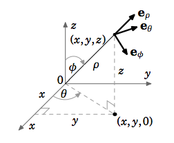
Similarly, a point $(x, y, z)$ can be represented in spherical coordinates $(ρ,θ,φ)$, where $x = ρ \sin φ \cos θ, y = ρ \sin φ \sin θ, z = ρ \cos φ.$ At each point $(ρ,θ,φ)$, let $\textbf{e}_ρ, \textbf{e}_θ, \textbf{e}_φ$ be unit vectors in the direction of increasing $ρ, θ, φ$, respectively (see Figure 4.6.2). Then the vectors $\textbf{e}_ρ, \textbf{e}_θ, \textbf{e}_φ$ are orthonormal. By the right-hand rule, we see that $\textbf{e}_θ × \textbf{e}_ρ = \textbf{e}_φ$.

We can now summarize the expressions for the gradient, divergence, curl and Laplacian in Cartesian, cylindrical and spherical coordinates in the following tables:

Cartesian

$(x, y, z)$: Scalar function $F$; Vector field $\textbf{f} = f_1 \textbf{i}+ f_2 \textbf{j}+ f_3\textbf{k}$

• gradient : $∇F = \dfrac{∂F}{ ∂x}\textbf{i} + \dfrac{∂F}{ ∂y}\textbf{j} + \dfrac{∂F}{ ∂z}\textbf{k}$
• divergence : $∇·\textbf{f} = \dfrac{∂f_1}{ ∂x} + \dfrac{∂f_2}{ ∂y} + \dfrac{∂f_3}{ ∂z}$
• curl : $∇ × \textbf{f} = \left ( \dfrac{∂f_3}{ ∂y} − \dfrac{∂f_2}{ ∂z} \right ) \textbf{i} + \left ( \dfrac{∂f_1}{ ∂z} − \dfrac{∂f_3}{ ∂x} \right ) \textbf{j} + \left ( \dfrac{∂f_2}{ ∂x} − \dfrac{∂f_1}{ ∂y} \right )\textbf{k}$
• Laplacian : $∆F = \dfrac{∂^ 2F}{ ∂x^ 2} + \dfrac{∂^ 2F}{ ∂y^ 2} + \dfrac{∂^ 2F}{ ∂z^ 2}$

Cylindrical

$(r,θ, z)$: Scalar function $F$; Vector field $\textbf{f} = f_r \textbf{e}_r + f_θ \textbf{e}_θ + f_z \textbf{e}_z$

• gradient : $∇F = \dfrac{∂F}{ ∂r} \textbf{e}_r + \dfrac{1}{ r}\dfrac{ ∂F}{ ∂θ} \textbf{e}_θ + \dfrac{∂F}{ ∂z} \textbf{e}_z$
• divergence : $∇·\textbf{f} = \dfrac{1}{ r}\dfrac{ ∂}{ ∂r} (r f_r) + \dfrac{1}{ r} \dfrac{∂f_θ}{ ∂θ} + \dfrac{∂f_z}{ ∂z}$
• curl : $∇ × \textbf{f} = \left ( \dfrac{1}{ r} \dfrac{∂f_z}{ ∂θ} − \dfrac{∂f_θ}{ ∂z} \right ) \textbf{e}_r + \left ( \dfrac{∂f_r}{ ∂z} − \dfrac{∂f_z}{ ∂r} \right ) \textbf{e}_θ + \dfrac{1}{ r} \left ( \dfrac{∂}{ ∂r} (r f_θ)− \dfrac{∂f_r}{ ∂θ}\right ) \textbf{e}_z$
• Laplacian : $∆F = \dfrac{1}{ r}\dfrac{ ∂}{ ∂r} \left ( r \dfrac{∂F}{ ∂r} \right ) + \dfrac{1}{ r^2} \dfrac{∂^ 2F}{ ∂θ^2} + \dfrac{∂^ 2F}{ ∂z^ 2}$

Spherical

$(ρ,θ,φ)$: Scalar function $F$; Vector field $\textbf{f} = f_ρ \textbf{e}_ρ + f_θ \textbf{e}_θ + f_φ \textbf{e}_φ$

• gradient : $∇F = \dfrac{∂F}{ ∂ρ} \textbf{e}_ρ + \dfrac{1}{ ρ \sin φ} \dfrac{∂F}{ ∂θ} \textbf{e}_θ + \dfrac{1}{ ρ}\dfrac{ ∂F}{ ∂φ} \textbf{e}_φ$
• divergence : $∇·\textbf{f} = \dfrac{1}{ ρ^ 2} \dfrac{∂}{ ∂ρ} (ρ^ 2 f_ρ) + \dfrac{1}{ ρ} \sin φ \dfrac{∂f_θ}{ ∂θ} + \dfrac{1}{ ρ \sin φ} \dfrac{∂}{ ∂φ} (\sin φ f_θ)$
• curl : $∇ × \textbf{f} = \dfrac{1}{ ρ \sin φ} \left ( \dfrac{∂}{ ∂φ} (\sin φ f_θ)− \dfrac{∂f_φ}{ ∂θ} \right ) \textbf{e}_ρ + \dfrac{1}{ ρ} \left ( \dfrac{∂}{ ∂ρ} (ρ f_φ)− \dfrac{∂f_ρ}{ ∂φ} \right ) \textbf{e}_θ + \left ( \dfrac{1}{ ρ \sin φ} \dfrac{∂f_ρ}{ ∂θ} − \dfrac{1}{ ρ} \dfrac{∂}{ ∂ρ} (ρ f_θ) \right ) \textbf{e}_φ$
• Laplacian : $∆F = \dfrac{1}{ ρ^ 2} \dfrac{∂}{ ∂ρ} \left ( ρ^ 2 \dfrac{∂F}{ ∂ρ} \right ) + \dfrac{1}{ ρ^ 2 \sin^2 φ} \dfrac{∂^ 2F}{ ∂θ^2} + \dfrac{1}{ ρ^ 2 \sin φ} \dfrac{∂}{ ∂φ} \left ( \sin φ \dfrac{∂F}{ ∂φ}\right )$

The derivation of the above formulas for cylindrical and spherical coordinates is straightforward but extremely tedious. The basic idea is to take the Cartesian equivalent of the quantity in question and to substitute into that formula using the appropriate coordinate transformation. As an example, we will derive the formula for the gradient in spherical coordinates.

Goal: Show that the gradient of a real-valued function $F(ρ,θ,φ)$ in spherical coordinates is:

$$\nonumber ∇F = \dfrac{∂F}{ ∂ρ} \textbf{e}_ρ + \dfrac{1}{ ρ \sin φ} \dfrac{∂F}{ ∂θ} \textbf{e}_θ +\dfrac{1}{ ρ}\dfrac{ ∂F}{ ∂φ}\textbf{e}_φ$$

Idea: In the Cartesian gradient formula $∇F(x, y, z) = \dfrac{∂F}{ ∂x}\textbf{i}+ \dfrac{∂F}{ ∂y}\textbf{j}+ \dfrac{∂F}{ ∂z}\textbf{k}$, put the Cartesian basis vectors i, j, k in terms of the spherical coordinate basis vectors $\textbf{e}_ρ, \textbf{e}_θ, \textbf{e}_φ$ and functions of $ρ, θ \text{ and }φ$. Then put the partial derivatives $\dfrac{∂F}{ ∂x} , \dfrac{∂F}{ ∂y} , \dfrac{∂F}{ ∂z}$ in terms of $\dfrac{∂F}{ ∂ρ} , \dfrac{∂F}{ ∂θ} , \dfrac{∂F}{ ∂φ}$ and functions of $ρ, θ \text{ and }φ$.

Step 1: Get formulas for $\textbf{e}_ρ, \textbf{e}_θ, \textbf{e}_φ$ in terms of i, j, k.

We can see from Figure 4.6.2 that the unit vector $\textbf{e}_ρ$ in the $ρ$ direction at a general point $(ρ,θ,φ)$ is $\textbf{e}_ρ = \dfrac{\textbf{r}}{ \lVert \textbf{r} \rVert } , \text{ where }\textbf{r} = x\textbf{i} + y\textbf{j} + z\textbf{k}$ is the position vector of the point in Cartesian coordinates. Thus,

$$\nonumber \textbf{e}_ρ = \dfrac{\textbf{r}}{ \lVert \textbf{r} \rVert} = \dfrac{x\textbf{i}+ y\textbf{j}+ z\textbf{k}}{ \sqrt{ x^ 2 + y^ 2 + z^ 2}} ,$$

so using $x = ρ \sin φ \cos θ, y = ρ \sin φ \sin θ, z = ρ \cos φ, \text{ and }ρ = \sqrt{ x^ 2 + y^ 2 + z^ 2}$, we get:

$$\nonumber \fbox{\(\textbf{e}_ρ = \sin φ \cos θ\textbf{i} + \sin φ \sin θ \textbf{j} + \cos φ\textbf{k}\)}$$

Now, since the angle $θ$ is measured in the $x y$-plane, then the unit vector $\textbf{e}_θ \text{ in the }θ$ direction must be parallel to the $x y$-plane. That is, $\textbf{e}_θ \text{ is of the form }a\textbf{i} + b\textbf{j} + 0\textbf{k}$. To figure out what $a \text{ and }b$ are, note that since $\textbf{e}_θ \perp \textbf{e}_ρ$, then in particular $\textbf{e}_θ \perp \textbf{e}_ρ$ when $\textbf{e}_ρ \text{ is in the }x y$-plane. That occurs when the angle $φ \text{ is }π/2$. Putting $φ = π/2$ into the formula for $\textbf{e}_ρ \text{ gives }\textbf{e}_ρ = \cos θ \textbf{i}+\sin θ \textbf{j}+0\textbf{k}$, and we see that a vector perpendicular to that is $−\sin θ \textbf{i}+\cos θ \textbf{j}+0\textbf{k}$. Since this vector is also a unit vector and points in the (positive) $θ$ direction, it must be $\textbf{e}_θ$:

$$\nonumber \fbox{\(\textbf{e}_θ = −\sin θ \textbf{i} + \cos θ \textbf{j} + 0\textbf{k}\)}$$

Lastly, since $\textbf{e}_φ = \textbf{e}_θ × \textbf{e}_ρ,$ we get:

$$\nonumber \fbox{\(\textbf{e}_φ = \cos φ \cos θ \textbf{i} + \cos φ \sin θ \textbf{j} − \sin φ\textbf{k}\)}$$

Step 2: Use the three formulas from Step 1 to solve for i, j, k in terms of $\textbf{e}_ρ, \textbf{e}_θ, \textbf{e}_φ$.

This comes down to solving a system of three equations in three unknowns. There are many ways of doing this, but we will do it by combining the formulas for $\textbf{e}_ρ \text{ and }\textbf{e}_φ \text{ to eliminate }k$, which will give us an equation involving just i and j. This, with the formula for $\textbf{e}_θ$, will then leave us with a system of two equations in two unknowns (i and j), which we will use to solve first for j then for i. Lastly, we will solve for k.

First, note that

$$\nonumber \sin φ \textbf{e}_ρ + \cos φ \textbf{e}_φ = \cos θ \textbf{i} + \sin θ \textbf{j}$$

so that

$$\nonumber \sin θ (\sin φ \textbf{e}_ρ + \cos φ \textbf{e}_φ) + \cos θ \textbf{e}_θ = (\sin^2 θ +\cos^2 θ)\textbf{j} = \textbf{j} ,$$

and so:

$$\nonumber \fbox{\(\textbf{j} = \sin φ \sin θ \textbf{e}_ρ + \cos θ \textbf{e}_θ + \cos φ \sin θ \textbf{e}_φ\)}$$

Likewise, we see that

$$\nonumber \cos θ (\sin φ \textbf{e}_ρ + \cos φ \textbf{e}_φ) − \sin θ \textbf{e}_θ = (\cos^2 θ +\sin^2 θ)\textbf{i} = \textbf{i} ,$$

and so:

$$\nonumber \fbox{\(\textbf{i} = \sin φ \cos θ \textbf{e}_ρ − \sin θ \textbf{e}_θ + \cos φ \cos θ \textbf{e}_φ\)}$$

Lastly, we see that:

$$\nonumber \fbox{\(\textbf{k} = \cos φ \textbf{e}_ρ − \sin φ \textbf{e}_φ\)}$$

Step 3: Get formulas for $\dfrac{∂F}{ ∂ρ} , \dfrac{∂F}{ ∂θ} , \dfrac{∂F}{ ∂φ} \text{ in terms of }\dfrac{∂F}{ ∂x} , \dfrac{∂F}{ ∂y} , \dfrac{∂F}{ ∂z}$.

By the Chain Rule, we have

$$\nonumber \begin{align} \dfrac{∂F}{ ∂ρ} &= \dfrac{∂F}{ ∂x} \dfrac{∂x}{ ∂ρ} + \dfrac{∂F}{ ∂y}\dfrac{ ∂y}{ ∂ρ} + \dfrac{∂F}{ ∂z} \dfrac{∂z}{ ∂ρ}, \\[4pt] \nonumber \dfrac{∂F}{ ∂θ} &= \dfrac{∂F}{ ∂x} \dfrac{∂x}{ ∂θ} + \dfrac{∂F}{ ∂y} \dfrac{∂y}{ ∂θ} + \dfrac{∂F}{ ∂z} \dfrac{∂z}{ ∂θ}, \\[4pt] \nonumber \dfrac{∂F}{ ∂φ} &= \dfrac{∂F}{ ∂x} \dfrac{∂x}{ ∂φ} + \dfrac{∂F}{ ∂y} \dfrac{∂y}{ ∂φ} + \dfrac{∂F}{ ∂z} \dfrac{∂z}{ ∂φ} ,\\[4pt] \end{align}$$

which yields:

$$\fbox{\(\nonumber \begin{align} \dfrac{∂F}{ ∂ρ} &= \sin φ \cos θ\dfrac{∂F}{ ∂x} + \sin φ \sin θ \dfrac{∂F}{ ∂y} + \cos φ \dfrac{∂F}{ ∂z} \\[4pt] \nonumber \dfrac{∂F}{ ∂θ} &= −ρ \sin φ \sin θ \dfrac{∂F}{ ∂x} + ρ \sin φ \cos θ \dfrac{∂F}{ ∂y} \\[4pt] \nonumber \dfrac{∂F}{ ∂φ} &= ρ \cos φ \cos θ \dfrac{∂F}{ ∂x} + ρ \cos φ \sin θ \dfrac{∂F}{ ∂y} − ρ \sin φ \dfrac{∂F}{ ∂z} \\[4pt] \end{align}\)}$$

Step 4: Use the three formulas from Step 3 to solve for $\dfrac{∂F}{ ∂x} , \dfrac{∂F}{ ∂y} , \dfrac{∂F}{ ∂z}$ in terms of $\dfrac{∂F}{ ∂ρ} , \dfrac{∂F}{ ∂θ} , \dfrac{∂F}{ ∂φ}$.

Again, this involves solving a system of three equations in three unknowns. Using a similar process of elimination as in Step 2, we get:

$$\fbox{\(\nonumber \begin{align}\dfrac{∂F}{ ∂x} &= \dfrac{1}{ ρ \sin φ} \left ( ρ \sin^2 φ \cos θ \dfrac{∂F}{ ∂ρ} − \sin θ \dfrac{∂F}{ ∂θ} + \sin φ \cos φ \cos θ \dfrac{∂F}{ ∂φ}\right ) \\[4pt] \nonumber \dfrac{∂F}{ ∂y} &= \dfrac{1}{ ρ \sin φ} \left ( ρ \sin^2 φ \sin θ \dfrac{∂F}{ ∂ρ} + \cos θ \dfrac{∂F}{ ∂θ} + \sin φ \cos φ \sin θ \dfrac{∂F}{ ∂φ}\right ) \\[4pt] \nonumber \dfrac{∂F}{ ∂z} &= \dfrac{1}{ρ} \left ( ρ \cos φ \dfrac{∂F}{ ∂ρ} − \sin φ \dfrac{∂F}{ ∂φ}\right ) \\[4pt] \end{align}\)}$$

Step 5: Substitute the formulas for i, j, k from Step 2 and the formulas for $\dfrac{∂F}{ ∂x} , \dfrac{∂F}{ ∂y} , \dfrac{∂F}{ ∂z}$ from Step 4 into the Cartesian gradient formula $∇F(x, y, z) = \dfrac{∂F}{ ∂x} \textbf{i}+ \dfrac{∂F}{ ∂y} \textbf{j}+ \dfrac{∂F}{ ∂z} \textbf{k}$.

Doing this last step is perhaps the most tedious, since it involves simplifying $3×3+3×3+ 2×2 = 22$ terms! Namely,

$$\nonumber \begin{align} ∇F &= \dfrac{1}{ ρ \sin φ} \left ( ρ \sin^2 φ \cos θ \dfrac{∂F}{ ∂ρ} −\sin θ \dfrac{∂F}{ ∂θ} +\sin φ \cos φ \cos θ \dfrac{∂F}{ ∂φ}\right ) (\sin φ \cos θ \textbf{e}_ρ −\sin θ \textbf{e}_θ +\cos φ \cos θ \textbf{e}_φ) \\[4pt] \nonumber &+\dfrac{1}{ ρ \sin φ} \left ( ρ \sin^2 φ \sin θ \dfrac{∂F}{ ∂ρ} +\cos θ \dfrac{∂F}{ ∂θ} +\sin φ \cos φ \sin θ \dfrac{∂F}{ ∂φ}\right ) (\sin φ \sin θ \textbf{e}_ρ +\cos θ \textbf{e}_θ +\cos φ \sin θ \textbf{e}_φ)\\[4pt] \nonumber &+\dfrac{1}{ ρ} \left ( ρ \cos φ \dfrac{∂F}{ ∂ρ} −\sin φ \dfrac{∂F}{ ∂φ}\right ) (\cos φ \textbf{e}_ρ −\sin φ \textbf{e}_φ) ,\\[4pt] \end{align}$$

which we see has 8 terms involving $\textbf{e}_ρ$, 6 terms involving $\textbf{e}_θ$, and 8 terms involving $\textbf{e}_φ$. But the algebra is straightforward and yields the desired result:

$$∇F = \dfrac{∂F}{ ∂ρ} \textbf{e}_ρ + \dfrac{1}{ ρ \sin φ} \dfrac{∂F}{ ∂θ} \textbf{e}_θ + \dfrac{1}{ ρ} \dfrac{∂F}{ ∂φ} \textbf{e}_φ \quad \checkmark$$

Example 4.19

In Example 4.17 we showed that $∇\lVert \textbf{r} \rVert ^2 = 2\textbf{r} \text{ and }∆\lVert \textbf{r} \rVert ^2 = 6, \text{ where }\textbf{r}(x, y, z) = x\textbf{i} + y\textbf{j} + z\textbf{k}$ in Cartesian coordinates. Verify that we get the same answers if we switch to spherical coordinates.

Solution

Since $\lVert \textbf{r} \rVert ^2 = x^ 2 + y^ 2 + z^ 2 = ρ^ 2 \text{ in spherical coordinates, let }F(ρ,θ,φ) = ρ^ 2$ (so that $F(ρ,θ,φ) = \lVert \textbf{r} \rVert ^2$ ). The gradient of $F$ in spherical coordinates is

$$\nonumber \begin{align} ∇F &= \dfrac{∂F}{ ∂ρ} \textbf{e}_ρ + \dfrac{1}{ ρ \sin φ} \dfrac{∂F}{ ∂θ} \textbf{e}_θ + \dfrac{1}{ ρ} \dfrac{∂F}{ ∂φ} \textbf{e}_φ \\[4pt] \nonumber &=2ρ \textbf{e}_ρ + \dfrac{1}{ ρ \sin φ} (0)\textbf{e}_θ + \dfrac{1}{ ρ} (0)\textbf{e}_φ \\[4pt] \nonumber &= 2ρ \textbf{e}_ρ = 2ρ \dfrac{\textbf{r}}{ \lVert \textbf{r} \rVert} , \text{ as we showed earlier, so}\\[4pt] \nonumber &= 2ρ \dfrac{\textbf{r}}{ ρ} = 2\textbf{r} , \text{ as expected. And the Laplacian is} \\[4pt] \nonumber ∆F &= \dfrac{1}{ ρ^ 2} \dfrac{∂}{ ∂ρ} \left ( ρ^2 \dfrac{∂F}{ ∂ρ} \right ) + \dfrac{1}{ ρ^ 2 \sin^2 φ} \dfrac{∂^2F}{ ∂θ^2} + \dfrac{1}{ ρ^ 2 \sin φ} \dfrac{∂}{ ∂φ} \left ( \sin φ \dfrac{∂F}{ ∂φ}\right ) \\[4pt] \nonumber &= \dfrac{1}{ ρ^ 2} \dfrac{∂}{ ∂ρ} (ρ^ 2 2ρ) + \dfrac{1}{ ρ^ 2 \sin φ} (0) + \dfrac{1}{ ρ^ 2 \sin φ} \dfrac{∂}{ ∂φ} \left ( \sin φ(0)\right ) \\[4pt] \nonumber &= \dfrac{1}{ ρ^ 2} \dfrac{∂}{ ∂ρ} (2ρ^ 3 ) + 0 + 0 \\[4pt] \nonumber &= \dfrac{1}{ ρ^ 2} (6ρ^ 2 ) = 6 , \text{ as expected.} \\[4pt] \end{align}$$