4.2: Probability measures

Okay, we’ve defined sample spaces and events, but when do quantitative notions like “the odds of" and “percent chance" come into play? They enter the scene when we define a probability measure. A probability measure is simply a function from the domain of events to the codomain of real numbers. We’ll normally use the letters “Pr" for our probability measure. In symbols, \(\text{Pr}:\mathbb{P}(\Omega) \to \mathbb{R}\) (since the set of all events is the power set of the sample space, as per above). There’s actually another constraint, though, which is that Pr’s values must be in the range 0 to 1, inclusive. So it’s more correct to write: \(\text{Pr}:\mathbb{P}(\Omega)\to [0,1]\). (You may recall from a previous math course that ‘[’ and ‘]’ are used to describe a closed interval in which the endpoints are included in the interval.)

The “meaning" of the probability measure is intuitive enough: it indicates how likely we think each event is to occur. In the baby example, if we say Pr({boy}) = .5, it means there’s a .5 probability (a.k.a., a 50% chance) that a male child will be born. In the game example, if we say Pr(\(M\)) = .667, if means there’s a two-thirds chance of me winning the right to go first. In all cases, a probability of 0 means “impossible to occur" and a probability of 1 means “absolutely certain to occur." In colloquial English, we most often use percentages to talk about these things: we’ll say “there’s a 60% chance Obama will win the election" rather than “there’s a .6 probability of Obama winning." The math’s a bit clumsier if we deal with percentages, though, so from now on we’ll get in the habit of using probabilities rather than ‘percent chances,’ and we’ll use values in the 0 to 1 range rather than 0 to 100.

I find the easiest way to think about probability measures is to start with the probabilities of the outcomes, not events. Each outcome has a specific probability of occuring. The probabilities of events logically flow from that just by using addition, as we’ll see in a moment.

For example, let’s imagine that Fox Broadcasting is producing a worldwide television event called All-time Idol, in which the yearly winners of American Idol throughout its history all compete against each other to be crowned the “All-time American Idol champion." The four contestants chosen for this competition, along with their musical genres, and age when originally appearing on the show, are as follows:

Kelly Clarkson (20): pop, rock, R&B
Fantasia Barrino (20): pop, R&B
Carrie Underwood (22): country
David Cook (26): rock

Entertainment shows, gossip columns, and People magazine are all abuzz in the weeks preceding the competition, to the point where a shrewd analyst can estimate the probabilities of each contestant winning. Our current best estimates are: Kelly .2, Fantasia .2, Carrie .1, and David .5.

Computing the probability for a specific event is just a matter of adding up the probabilities of its outcomes. Define \(F\) as the event that a woman wins the competition. Clearly Pr(\(F\)) = .5, since Pr({Kelly}) = .2, Pr({Fantasia}) = .2, and Pr({Carrie}) = .1. If \(P\) is the event that a rock singer wins, Pr(\(P\)) = .7, since this is the sum of Kelly’s and David’s probabilities.

Now it turns out that not just any function will do as a probability measure, even if the domain (events) and codomain (real numbers in the range[0,1]) are correct. In order for a function to be a “valid" probability measure, it must satisfy several other rules:

1. [somethinghappens] \(\text{Pr}(\Omega) = 1\)

2. [nonegs] \(\text{Pr}(A) \geq 0\) for all \(A \subseteq \Omega\)

3. [probunion] \(\text{Pr}(A \cup B) = \text{Pr}(A) + \text{Pr}(B) - \text{Pr}(A \cap B)\)

Rule 1 basically means “something has to happen." If we create an event that includes every possible outcome, then there’s a probability of 1 (100% chance) the event will occur, because after all some outcome has got to occur. (And of course Pr(\(\Omega\)) can’t be greater than 1, either, because it doesn’t make sense to have any probability over 1.) Rule 2 says there’s no negative probabilities: you can’t define any event, no matter how remote, that has a less than zero chance of happening.

Rule 3 is called the “additivity property," and is a bit more difficult to get your head around. A diagram works wonders. Consider Figure [venn], called a “Venn diagram," which visually depicts sets and their contents. Here we have defined three events: \(F\) (as above) is the event that the winner is a woman; \(R\) is the event that the winner is a rock musician (perhaps in addition to other musical genres); and \(U\) is the event that the winner is underage (i.e., becomes a multimillionare before they can legally drink). Each of these events is depicted as a closed curve which encloses the outcomes that belong to it. There is obviously a great deal of overlap.

Now back to rule 3. Suppose I ask “what’s the probability that the All-time Idol winner is underage or a rock star?" Right away we face an irritating ambiguity in the English language: does “or" mean “either underage or a rock star, but not both?" Or does it mean “underage and/or rock star?" The former interpretation is called an exclusive or and the latter an inclusive or. In computer science, we will almost always be assuming an inclusive or, unless explicitly noted otherwise.

Figure \(\PageIndex{1}\): Various events, and their overlap.

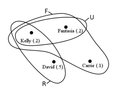
Very well then. What we’re really asking here is “what’s Pr(\(U \cup R\))?" We want the union of the two events, since we’re asking for the probability that either (or both) of them occurs. You might first think that we’d add the two probabilities for the two events and be done with it, but a glance at the diagram tells you this means trouble. Pr(\(U\)) is .4, and Pr(\(R\)) is .7. Even if we weren’t very smart, we’d know something was wrong as soon as we added \(.4 + .7 = 1.1\) to get a probability of over 1 and violate rule 1. But we are smart, and looking at the diagram it’s easy to see what happened: we double-counted Kelly’s probability. Kelly was a member of both groups, so her .2 got counted in there twice. Now you can see the rationale for rule 3. To get Pr(\(U \cup R\)) we add Pr(\(U\)) and Pr(\(R\)), but then we have to subtract back out the part we double-counted. And what did we double-count? Precisely the intersection \(U \cap R\).

As a second example, suppose we want the probability of an underage or female winner? Pr(\(U\)) = .4, and Pr(\(F\)) = .5, so the first step is to just add these. Then we subtract out the intersection, which we double counted. In this case, the intersection \(U \cap F\) is just \(U\) (check the diagram), and so subtract out the whole .4. The answer is .5, as it should be.

By the way, you’ll notice that if the two sets in question are mutually exclusive, then there is no intersection to subtract out. That’s a special case of rule 3. For example, suppose I defined the event \(C\) as a country singer winning the competition. In this case, \(C\) contains only one outcome: Carrie. Therefore \(U\) and \(C\) are mutually exclusive. So if I asked “what’s the probability of an underage or country winner?" we’d compute Pr(\(U \cup C\)) as

\[\begin{aligned} \text{Pr}(U \cup C) &= \text{Pr}(U) + \text{Pr}(C) - \text{Pr}(U \cap C) \\ &= .4 + .1 - 0 \\ &= .5.\end{aligned}\]

We didn’t double-count anything, so there was no correction to make.

Here are a few more pretty obvious rules for probability measures, which follow logically from the first 3:

4. Pr(\(\varnothing\)) = 0

5. Pr(\(\overline{A}\)) = \(1-\)Pr(\(A\)) (recall the “total complement" operator from p. .)

6. Pr(\(A\)) \(\leq\) Pr(\(B\)) if \(A \subseteq B\)

Finally, let me draw attention to a common special case of the above rules, which is the situation in which all outcomes are equally likely. This usually happens when we roll dice, flip coins, deal cards, etc. since the probability of rolling a 3 is (normally) the same as rolling a 6, and the probability of being dealt the 10\(\spadesuit\) is the same as the Q\(\diamondsuit\). It may also happen when we generate encryption keys, choose between alternate network routing paths, or determine the initial positions of baddies in a first-person shooter level.

In this case, if there are \(N\) possible outcomes (note \(N=|\Omega|\)) then the probability of any event A is:

Pr(\(A\)) = \(\dfrac{|A|}{N}\).

It’s the size (cardinality) of the event set that matters, and the ratio of this number to the total number of events is the probability. For example, if we deal a card from a fair deck, the probability of drawing a face card is

\[\begin{aligned} \text{Pr}(F) &= \frac{|F|}{N} \\[.1in] &= \frac{|\{K\spadesuit,K\heartsuit,K\diamondsuit,\cdots,J\clubsuit\}|}{52} \\[.1in] &= \frac{12}{52} = .231.\end{aligned}\]

Please realize that this shortcut only applies when the probability of each outcome is the same. We certainly couldn’t say, for example, that the probability of a user’s password starting with the letter q is just \(\frac{1}{26}\), because passwords surely don’t contain all letters with equal frequency. (At least, I’d be very surprised if that were the case.) The only way to solve a problem like this is to know how often each letter of the alphabet occurs.