6.3: Combinations

All the stuff with permutations has emphasized order. Somebody gets first place in the golf tournament, and somebody else gets second, and you bet your bottom dollar that it matters which is which. What if it turns out we don’t care about the order, though? Maybe we don’t care who got what place, but just which golfers were in the top ten. Maybe we don’t care which film is showing in which time slot, but only which films are in tonight’s movie lineup.

This counting scenario involves something called combinations rather than permutations. A combination of \(k\) objects out of a possible \(n\) is a choice of any set of \(k\) of them, without regard to order. For instance, suppose all three Davies kids want to play on the Wii, but only two can play at a time. Who will get to play first after school? One possibility is Lizzy and T.J., another is Lizzy and Johnny, and the last one is T.J. and Johnny. These are the three (and only three) combinations of 2 objects out of 3.

To see how to count these in general, let’s return to the golf tournament example. Suppose that in addition to winning money, the top three finishers of our local tournament will also advance to the regional tournament. This is a great honor, and brings with it far greater additional winning potential than the local money did. Question: how many different possible trios might we send to regional competition?

At first glance, this seems just like the “how many prize money allocations" problem from before, except that we’re taking 3 instead of 10. But there is a twist. In the former problem, it mattered who was first vs. second vs. third. Now the order is irrelevant. If you finish in the top three, you advance, period. You don’t “advance more forcefully" for finishing first locally instead of third.

It’s not as obvious how to count this, but of course there is a trick. The trick is to count the partial permutations, but then realize how much we overcounted, and then compensate for it accordingly.

If we count the partial permutations of 3 out of 45 golfers, we have \(45^{\underline{3}}\) such permutations. One of those partial permutations is:

1.Phil  2.Bubba  3.Tiger

Another one is:

1.Phil  2.Tiger  3.Bubba

and yet another is:

1.Tiger  2.Phil  3.Bubba

Now the important thing to recognize is that in our present problem — counting the possible number of regional-bound golf trios — all three of these different partial permutations represent the same combination. In all three cases, it’s Bubba, Phil, and Tiger who will represent our local golf association in the regional competition. So by counting all three of them as separate partial permutations, we’ve overcounted the combinations.

Obviously we want to count Bubba/Phil/Tiger only once. Okay then. How many times did we overcount it when we counted partial permutations? The answer is that we counted this trio once for every way it can be permuted. The three permutations, above, were examples of this, and so are these three:

1.Tiger  2.Bubba  3.Phil
1.Bubba  2.Tiger  3.Phil
1.Bubba  2.Phil  3.Tiger

This makes a total of six times that we (redundantly) counted the same combination when we counted the partial permutations. Why 6? Because that’s the value of 3!, of course. There are 3! different ways to arrange Bubba, Phil, and Tiger, since that’s just a straight permutation of three elements. And so we find that every threesome we want to account for, we have counted 6 times.

The way to get the correct answer, then, is obviously to correct for this overcounting by dividing by 6: \[\dfrac{45^{\underline{3}}}{3!} = \dfrac{45 \times 44 \times 43}{6} = \text{14,190 different threesomes}.\] And in general, that’s all we have to do. To find the number of combinations of \(k\) things taken from a total of \(n\) things we have: \[\dfrac{n^{\underline{k}}}{k!} = \dfrac{n!}{(n-k)!k!}\ \text{combinations}.\] This pattern, too, comes up so often that mathematicians have invented (yet) another special notation for it. It looks a bit strange at first, almost like a fraction without a horizontal bar: \[\binom{n}{k} = \dfrac{n!}{(n-k)!k!}.\] This is pronounced “\(n\)-choose-\(k\)".

Again, examples abound. How many different 5-card poker hands are there? Answer: \(\binom{52}{5}\), since it doesn’t matter what order you’re dealt the cards, only which five cards you get. If there are 1024 sectors on our disk, but only 256 cache blocks in memory to hold them, how many different combinations of sectors can be in memory at one time? \(\binom{1024}{256}\). If we want to choose 4 or 5 of our top 10 customers to participate in a focus group, how many different combinations of participants could we have? \(\binom{10}{4}+\binom{10}{5}\), since we want the number of ways to pick 4 of them plus the number of ways to pick 5 of them. And for our late night movie channel, of course, there are \(\binom{500}{4}\) possible movie lineups to attract audiences, if we don’t care which film is aired at which time.

Binomial coefficients

The “n-choose-k" notation \(\binom{n}{k}\) has another name: values of this sort are called binomial coefficients. This is because one way to generate them, believe it or not, is to repeatedly multiply a binomial times itself (or, equivalently, take a binomial to a power.)

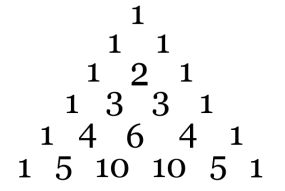
A binomial, recall, is a polynomial with just two terms: \[x+y.\] The coefficients for this binomial are of course 1 and 1, since “\(x\)" really means “\(1\cdot x\)." Now if we multiply this by itself, we get: \[\begin{aligned} (x+y)\cdot(x+y) = x^2 + 2xy + y^2.\end{aligned}\] The coefficients of the terms being 1, 2, and 1. We do it again: \[\begin{aligned} (x^2+2xy+y^2)\cdot(x+y) = x^3 + 3x^2y + 3xy^2 + y^3.\end{aligned}\] to get 1, 3, 3, and 1, and do it again: \[\begin{aligned} (x^3+3x^2y+3xy^2+y^3)\cdot(x+y) = x^4 + 4x^3y + 6x^2y^2 + 4xy^3 + y^4.\end{aligned}\] to get 1, 4, 6, 4, and 1. At this point you might be having flashbacks to Pascal’s triangle, which perhaps you learned about in grade school, in which each entry in a row is the sum of the two entries immediately above it (to the left and right), as in Figure \(\PageIndex{1}\). (If you never learned that, don’t worry about it.)

Figure \(\PageIndex{1}\): The first six rows of Pascal’s triangle.

Now you might be wondering where I’m going with this. What do fun algebra tricks have to do with counting combinations of items? The answer is that the values of \(\binom{n}{k}\) are precisely the coefficients of these multiplied polynomials. Let \(n\) be 4, which corresponds to the last polynomial we multiplied out. We can then compute all the combinations of items taken from a group of four: \[\binom{4}{0}=1, \binom{4}{1}=4, \binom{4}{2}=6, \binom{4}{3}=4, \text{and}\ \binom{4}{4}=1.\] In other words, there is exactly one way of taking no items out of 4 (you simply don’t take any). There are four ways of taking one item out of 4 — you could take the first, or the second, or the third, or the fourth. There are six ways of taking two items out of four; namely:

1. the first and second
2. the first and third
3. the first and fourth
4. the second and third
5. the second and fourth
6. the third and fourth

And so on.

Now in some ways we’re on a bit of a tangent, since the fact that the “n-choose-k" values happen to work out to be the same as the binomial coefficients is mostly just an interesting coincidence. But what I really want you to take notice of here — and what Pascal’s triangle makes plain — is the symmetry of the coefficients. This surprises a lot of students. What if I asked you which of the following numbers was greater: \(\binom{1000}{18}\) or \(\binom{1000}{982}\)? Most students guess that the second of these numbers is far greater. In actual fact, though, they both work out to \(\frac{1000!}{18!982!}\) and are thus exactly the same. And in the above example, we see that \(\binom{4}{0}\) is equal to \(\binom{4}{4}\), and that \(\binom{4}{1}\) is equal to \(\binom{4}{3}\).

Why is this? Well, you can look back at the formula for \(\binom{n}{k}\) and see how it works out algebraically. But it’s good to have an intuitive feel for it as well. Here’s how I think of it. Go back to the Davies kids and the Wii. We said there were three different ways to choose 2 kids to play on the Wii first after school. In other words, \(\binom{3}{2} = 3.\) Very well. But if you think about it, there must then also be three different ways to leave out exactly one kid. If we change what we’re counting from “combinations of players" to “combinations of non-players" — both of which must be equal, since no matter what happens, we’ll be partitioning the Davies kids into players and non-players — then we see that \(\binom{3}{1}\) must also be 3.

And this is true across the board. If there are \(\binom{500}{4}\) different lineups of four movies, then there are the same number of lineups of 496 movies, since \(\binom{500}{4} = \binom{500}{496}\). Conceptually, in the first case we choose a group of four and show them, and in the second case we choose a group of four and show everything but them.

Also notice that the way to get the greatest number of combinations of \(n\) items is for \(k\) to be half of \(n\). If we have 100 books in our library, there are a lot more ways to check out 50 of them then there are to check out only 5, or to check out 95. Strange but true.

Lastly, make sure you understand the extreme endpoints of this phenomenon. \(\binom{n}{0}\) and \(\binom{n}{n}\) are both always 1, no matter what \(n\) is. That’s because if you’re picking no items, you have no choices at all: there’s only one way to come up empty. And if you’re picking all the items, you also have no choices: you’re forced to pick everything.