
10.1: An Introduction to Probability
- Page ID
- 97925

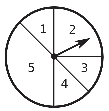
We continue with an informal discussion intended to motivate the more structured development that will follow. Consider the “spinner” shown in Figure 10.1. Suppose we give it a good thwack so that the arrow goes round and round. We then record the number of the region in which the pointer comes to rest. Then observers, none of whom have studied combinatorics, might make the following comments:
- The odds of landing in region 1 are the same as those for landing in region 3.
- You are twice as likely to land in region 2 as in region 4.
- When you land in an odd numbered region, then 60% of the time, it will be in region 5.
We will now develop a more formal framework that will enable us to make such discussions far more precise. We will also see whether Alice is being entirely fair to Bob in her proposed game to one hundred.
We begin by defining a probability space as a pair \((S,P)\) where \(S\) is a finite set and \(P\) is a function that whose domain is the family of all subsets of \(S\) and whose range is the set [0,1] of all real numbers which are non-negative and at most one. Furthermore, the following two key properties must be satisfied:
- \(P(\emptyset) = 0\) and \(P(S) = 1\).
- If \(A\) and \(B\) are subsets of \(S\), and \(A \cap B= \emptyset\), then \(P(A \cup B) = P(A) + P(B)\).
When \((S,P)\) is a probability space, the function \(P\) is called a probability measure, the subsets of \(S\) are called events, and when \(E⊆S\), the quantity \(P(E)\) is referred to as the probability of the event \(E\).
Note that we can consider \(P\) to be extended to a mapping from \(S\) to [0,1] by setting \(P(x)=P(\{x\})\) for each element \(x \in S\). We call the elements of \(S\) outcomes (some people prefer to say the elements are elementary outcomes) and the quantity \(P(x)\) is called the probability of \(x\). It is important to realize that if you know \(P(x)\) for each \(x \in S\), then you can calculate \(P(E)\) for any event \(E\), since (by the second property), \(P(E) = \sum_{x \in X} P(x)\).
For the spinner, we can take \(S=\{1,2,3,4,5\}\), with \(P(1)=P(3)=P(4)=1/8, P(2)=2/8=1/4\) and \(P(5)=3/8\). So \(P(\{2,3\}) = 1/8 + 2/8 = 3/8\).
Let \(S\) be a finite, nonempty set and let \(n=|S|\). For each \(E⊆S\), set \(P(E)=|E|/n\). In particular, \(P(x)=1/n\) for each element \(x \in S\). In this trivial example, all outcomes are equally likely.
If a single six sided die is rolled and the number of dots on the top face is recorded, then the ground set is \(S=\{1,2,3,4,5,6\}\) and \(P(i)=1/6\) for each \(i \in S\). On the other hand, if a pair of dice are rolled and the sum of the dots on the two top faces is recorded, then \(S=\{2,3,4,…,11,12\}\) with \(P(2)=P(12)=1/36, P(3)=P(11)=2/36, P(4)=P(10)=3/36, P(5)=P(9)=4/36, P(6)=P(8)=5/36\) and \(P(7)=6/36\). To see this, consider the two die as distinguished, one die red and the other one blue. Then each of the pairs \((i,j)\) with \(1 \leq i,j \leq 6\), the red die showing \(i\) spots and the blue die showing \(j\) spots is equally likely. So each has probability 1/36. Then, for example, there are three pairs that yield a total of four, namely (3,1), (2,2) and (1,3). So the probability of rolling a four is 3/36=1/12.
In Alice's game as described above, the set \(S\) can be {0,1,2,3,4,5}, the set of possible differences when a pair of dice are rolled. In this game, we will see that the correct definition of the function \(P\) will set \(P(0)=6/36; P(1)=10/36; P(2)=8/36; P(3)=6/36; P(4)=4/36\); and \(P(5)=2/36\). Using Xing's more compact notation, we could say that \(P(0)=1/6\) and \(P(d)=2(6−d)/36\) when \(d > 0\).
A jar contains twenty marbles, of which six are red, nine are blue and the remaining five are green. Three of the twenty marbles are selected at random. Let \(X=\{0,1,2,3,4,5\}\), and for each \(x \in X\), let \(P(x)\) denote the probability that the number of blue marbles among the three marbles selected is \(x\). Then \(P(i)=C(9,i)C(11,3−i)/C(20,3)\) for \(i=0,1,2,3\), while \(P(4)=P(5)=0\). Bob says that it doesn't make sense to have outcomes with probability zero, but Carlos says that it does.
In some cards games, each player receives five cards from a standard deck of 52 cards—four suits (spades, hearts, diamonds and clubs) with 13 cards, ace though king in each suit. A player has a full house if there are two values \(x\) and \(y\) for which he has three of the four \(x\)'s and two of the four \(y\)'s, e.g. three kings and two eights. If five cards are drawn at random from a standard deck, the probability of a full house is
\(\dfrac{\binom{13}{1} \binom{12}{1} \binom{4}{3} \binom{4}{2}}{\binom{52}{5}} \approx 0.00144\)