13.3: Augmenting Paths

In this section, we develop the classic labeling algorithm of Ford and Fulkerson which starts with any flow in a network and proceeds to modify the flow—always increasing the value of the flow—until reaching a step where no further improvements are possible. The algorithm will also help resolve the debate Alice, Bob, Carlos, and Yolanda were having in the previous section.

Our presentation of the labeling algorithm makes use of some natural and quite descriptive terminology. Suppose we have a network \(\textbf{G}=(V,E)\) with a flow \(ϕ\) of value \(v\). We call \(ϕ\) the current flow and look for ways to augment \(ϕ\) by making a relatively small number of changes. An edge \((x,y)\) with \(ϕ(x,y)>0\) is said to be used, and when \(ϕ(x,y)=c(x,y)>0\), we say the edge is full. When \(ϕ(x,y)<c(x,y)\), we say the edge \((x,y)\) has spare capacity, and when \(0=ϕ(x,y)<c(x,y)\), we say the edge \((x,y)\) is empty. Note that we simply ignore edges with zero capacity.

The key tool in modifying a network flow is a special type of path, and these paths are not necessarily directed paths. An augmenting path is a sequence \(P=(x_0,x_1,…,x_m)\) of distinct vertices in the network such that \(x_0=S, x_m=T\), and for each \(i=1,2,…,m\), either

1. \((x_{i−1},x_i)\) has spare capacity or
2. \((x_i,x_{i−1})\) is used.

When condition (Item a) holds, it is customary to refer to the edge \((x_{i−1},x_i)\) as a forward edge of the augmenting path \(P\). Similarly, if condition (Item b) holds, then the (nondirected) edge \((x_{i−1},x_i)\) is called a backward edge since the path moves from \(x_{i−1}\) to \(x_i\), which is opposite the direction of the edge.

Example 13.6

Let's look again at the network and flow in Figure 13.2. The sequence of vertices \((S,F,A,T)\) meets the criteria to be an augmenting path, and each edge in it is a forward edge. Notice that increasing the flow on each of \((S,F), (F,A)\), and \((A,T)\) by any positive amount \(δ≤12\) results in increasing the value of the flow and preserves the conservation laws.

If our first example jumped out at you as an augmenting path, it's probably less clear at a quick glance that \((S,E,D,C,B,A,T)\) is also an augmenting path. All of the edges are forward edges except for \((C,B)\), since it's actually \((B,C)\) that is a directed edge in the network. Don't worry if it's not clear how this path can be used to increase the value of the flow in the network, as that's our next topic.

Ignoring, for the moment, the issue of finding augmenting paths, let's see how they can be used to modify the current flow in a way that increases its value by some \(δ>0\). Here's how for an augmenting path \(P=(x_0,x_1,…,x_m)\). First, let \(δ_1\) be the positive number defined by:

\(δ_1=min\{c(x_{i−1},x_i)−ϕ(x_{i−1},x_i):(x_{i−1},x_i)\) a forward edge of \(P\).}

The quantity \(c(x_{i−1},x_i)−ϕ(x_{i−1},x_i)\) is nothing but the spare capacity on the edge \((x_{i−1},x_i)\), and thus \(δ_1\) is the largest amount by which all of the forward edges of \(P\). Note that the edges \((x_0,x_1)\) and \((x_{m−1},x_m)\) are always forward edges, so the positive quantity \(δ_1\) is defined for every augmenting path.

When the augmenting path \(P\) has no backward edges, we set \(δ=δ_1\). But when \(P\) has one or more backward edges, we pause to set

\(δ_2=min\{ϕ(x_i,x_{i−1}):(x_{i−1},x_i)\) a backward edge of \(P\)}.

Since every backward edge is used, \(δ_2>0\) whenever we need to define it. We then set \(δ=min\{δ_1,δ_2\}\).

In either case, we now have a positive number \(δ\) and we make the following elementary observation, for which you are asked to provide a proof in Exercise 13.7.4.

Proposition 13.7

Suppose we have an augmenting path \(P=(x_0,x_1,…,x_m)\) with \(δ>0\) calculated as above. Modify the flow \(ϕ\) by changing the values along the edges of the path \(P\) by an amount which is either \(+δ\) or \(−δ\) according to the following rules:

1. Increase the flow along the edges of \(P\) which are forwards.
2. Decrease the flow along the edges of \(P\) which are backwards.

Then the resulting function \(\hat{ϕ}\) is a flow and it has value \(δ\).

Example 13.8

The network flow shown in Figure 13.2 has many augmenting paths. We already saw two of them in Example 13.6, which we call \(P_1\) and \(P_3\) below. In the list below, be sure you understand why each path is an augmenting path and how the value of \(δ\) is determined for each path.

1. \(P_1=(S,F,A,T)\) with \(δ=12\). All edges are forward.
2. \(P_2=(S,B,A,T)\) with \(δ=8\). All edges are forward.
3. \(P_3=(S,E,D,C,B,A,T)\) with \(δ=9\). All edges are forward, except \((C,B)\) which is backward.
4. \(P_4=(S,B,E,D,C,A,T)\) with \(δ=2\). All edges are forward, except \((B,E)\) and \((C,A)\) which are backward.

In Exercise 13.7.7, you are asked to update the flow in Figure 13.2 for each of these four paths individually.

13.3.1 Caution on Augmenting Paths

Bob's gotten really good at using augmenting paths to increase the value of a network flow. He's not sure how to find them quite yet, but he knows a good thing when he sees it. He's inclined to think that any augmenting path will be a good deal in his quest for a maximum-valued flow. Carlos is pleased about Bob's enthusiasm for network flows but is beginning to think that he should warn Bob about the dangers in using just any old augmenting path to update a network flow. They agree that the best situation is when the number of updates that need to be made is small in terms of the number of vertices in the network and that the size of the capacities on the edges and the value of a maximum flow should not have a role in the number of updates.

Bob says he can't see any way that the edge capacities could create a situation where a network with only a few vertices requires many updates, Carlos is thinking that an example is in order. He asks Bob to pick his favorite very large integer and to call it \(M\). He then draws the network on four vertices shown in Figure 13.9. Bob quickly recognizes that the maximum value of a flow in this network is \(2M\). He does this using the flow with \(ϕ(S,A)=M, ϕ(A,T)=M, ϕ(S,B)=M, ϕ(B,T)=M\) and \(ϕ(A,B)=0\). Carlos is pleased with Bob's work.

Figure 13.9. A Small Network

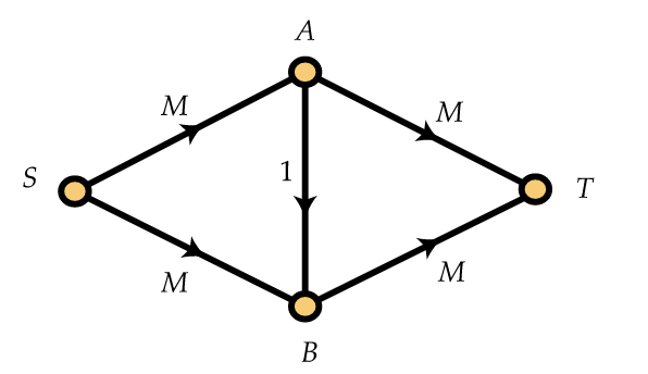
Since this network is really small, it was easy for Bob to find the maximum flow. However, Bob and Carlos agree that “eyeballing” is not an approach that scales well to larger networks, so they need to have an approach to finding that flow using augmenting paths. Bob tells Carlos to give him an augmenting path, and he'll do the updating. Carlos suggests the augmenting path \((S,A,B,T)\), and Bob determines that \(δ=1\) for this augmenting path. He updates the network (starting from the zero flow, i.e., with \(ϕ(e)=0\) for every edge \(e\)) and it now has value 1. Bob asks Carlos for another augmenting path, so Carlos gives him \((S,B,A,T)\). Now \((B,A)\) is backward, but that doesn't phase Bob. He performs the update, obtaining a flow of value 2 with \((A,B)\) empty again.

Despite Carlos' hope that Bob could already see where this was heading, Bob eagerly asks for another augmenting path. Carlos promptly gives him \((S,A,B,T)\), which again has \(δ=1\). Bob's update gives them a flow of value 3. Before Carlos can suggest another augmenting path, Bob realizes what the problem is. He points out that Carlos can just give him \((S,B,A,T)\) again, which will still have \(δ=1\) and result in the flow value increasing to 4. He says that they could keep alternating between those two augmenting paths, increasing the flow value by 1 each time, until they'd made \(2M\) updates to finally have a flow of value \(2M\). Since the network only has four vertices and \(M\) is very large, he realizes that using any old augmenting path is definitely not a good idea.

Carlos leaves Bob to try to figure out a better approach. He realizes that starting from the zero flow, he'd only need the augmenting paths \((S,A,T)\) and \((S,B,T)\), each with \(δ=M\) to quickly get the maximum flow. However, he's not sure why an algorithm should find those augmenting paths to be preferable. About this time, Dave wanders by and mumbles something about the better augmenting paths using only two edges, while Carlos' two evil augmenting paths each used three. Bob thinks that maybe Dave's onto something, so he decides to go back to reading his textbook.