Mathematics LibreTexts

17.1.1: An Introduction to Algorithms

  • Page ID
    81812
  • \( \newcommand{\vecs}[1]{\overset { \scriptstyle \rightharpoonup} {\mathbf{#1}} } \)

    \( \newcommand{\vecd}[1]{\overset{-\!-\!\rightharpoonup}{\vphantom{a}\smash {#1}}} \)

    \( \newcommand{\id}{\mathrm{id}}\) \( \newcommand{\Span}{\mathrm{span}}\)

    ( \newcommand{\kernel}{\mathrm{null}\,}\) \( \newcommand{\range}{\mathrm{range}\,}\)

    \( \newcommand{\RealPart}{\mathrm{Re}}\) \( \newcommand{\ImaginaryPart}{\mathrm{Im}}\)

    \( \newcommand{\Argument}{\mathrm{Arg}}\) \( \newcommand{\norm}[1]{\| #1 \|}\)

    \( \newcommand{\inner}[2]{\langle #1, #2 \rangle}\)

    \( \newcommand{\Span}{\mathrm{span}}\)

    \( \newcommand{\id}{\mathrm{id}}\)

    \( \newcommand{\Span}{\mathrm{span}}\)

    \( \newcommand{\kernel}{\mathrm{null}\,}\)

    \( \newcommand{\range}{\mathrm{range}\,}\)

    \( \newcommand{\RealPart}{\mathrm{Re}}\)

    \( \newcommand{\ImaginaryPart}{\mathrm{Im}}\)

    \( \newcommand{\Argument}{\mathrm{Arg}}\)

    \( \newcommand{\norm}[1]{\| #1 \|}\)

    \( \newcommand{\inner}[2]{\langle #1, #2 \rangle}\)

    \( \newcommand{\Span}{\mathrm{span}}\) \( \newcommand{\AA}{\unicode[.8,0]{x212B}}\)

    \( \newcommand{\vectorA}[1]{\vec{#1}}      % arrow\)

    \( \newcommand{\vectorAt}[1]{\vec{\text{#1}}}      % arrow\)

    \( \newcommand{\vectorB}[1]{\overset { \scriptstyle \rightharpoonup} {\mathbf{#1}} } \)

    \( \newcommand{\vectorC}[1]{\textbf{#1}} \)

    \( \newcommand{\vectorD}[1]{\overrightarrow{#1}} \)

    \( \newcommand{\vectorDt}[1]{\overrightarrow{\text{#1}}} \)

    \( \newcommand{\vectE}[1]{\overset{-\!-\!\rightharpoonup}{\vphantom{a}\smash{\mathbf {#1}}}} \)

    \( \newcommand{\vecs}[1]{\overset { \scriptstyle \rightharpoonup} {\mathbf{#1}} } \)

    \( \newcommand{\vecd}[1]{\overset{-\!-\!\rightharpoonup}{\vphantom{a}\smash {#1}}} \)

    \(\newcommand{\avec}{\mathbf a}\) \(\newcommand{\bvec}{\mathbf b}\) \(\newcommand{\cvec}{\mathbf c}\) \(\newcommand{\dvec}{\mathbf d}\) \(\newcommand{\dtil}{\widetilde{\mathbf d}}\) \(\newcommand{\evec}{\mathbf e}\) \(\newcommand{\fvec}{\mathbf f}\) \(\newcommand{\nvec}{\mathbf n}\) \(\newcommand{\pvec}{\mathbf p}\) \(\newcommand{\qvec}{\mathbf q}\) \(\newcommand{\svec}{\mathbf s}\) \(\newcommand{\tvec}{\mathbf t}\) \(\newcommand{\uvec}{\mathbf u}\) \(\newcommand{\vvec}{\mathbf v}\) \(\newcommand{\wvec}{\mathbf w}\) \(\newcommand{\xvec}{\mathbf x}\) \(\newcommand{\yvec}{\mathbf y}\) \(\newcommand{\zvec}{\mathbf z}\) \(\newcommand{\rvec}{\mathbf r}\) \(\newcommand{\mvec}{\mathbf m}\) \(\newcommand{\zerovec}{\mathbf 0}\) \(\newcommand{\onevec}{\mathbf 1}\) \(\newcommand{\real}{\mathbb R}\) \(\newcommand{\twovec}[2]{\left[\begin{array}{r}#1 \\ #2 \end{array}\right]}\) \(\newcommand{\ctwovec}[2]{\left[\begin{array}{c}#1 \\ #2 \end{array}\right]}\) \(\newcommand{\threevec}[3]{\left[\begin{array}{r}#1 \\ #2 \\ #3 \end{array}\right]}\) \(\newcommand{\cthreevec}[3]{\left[\begin{array}{c}#1 \\ #2 \\ #3 \end{array}\right]}\) \(\newcommand{\fourvec}[4]{\left[\begin{array}{r}#1 \\ #2 \\ #3 \\ #4 \end{array}\right]}\) \(\newcommand{\cfourvec}[4]{\left[\begin{array}{c}#1 \\ #2 \\ #3 \\ #4 \end{array}\right]}\) \(\newcommand{\fivevec}[5]{\left[\begin{array}{r}#1 \\ #2 \\ #3 \\ #4 \\ #5 \\ \end{array}\right]}\) \(\newcommand{\cfivevec}[5]{\left[\begin{array}{c}#1 \\ #2 \\ #3 \\ #4 \\ #5 \\ \end{array}\right]}\) \(\newcommand{\mattwo}[4]{\left[\begin{array}{rr}#1 \amp #2 \\ #3 \amp #4 \\ \end{array}\right]}\) \(\newcommand{\laspan}[1]{\text{Span}\{#1\}}\) \(\newcommand{\bcal}{\cal B}\) \(\newcommand{\ccal}{\cal C}\) \(\newcommand{\scal}{\cal S}\) \(\newcommand{\wcal}{\cal W}\) \(\newcommand{\ecal}{\cal E}\) \(\newcommand{\coords}[2]{\left\{#1\right\}_{#2}}\) \(\newcommand{\gray}[1]{\color{gray}{#1}}\) \(\newcommand{\lgray}[1]{\color{lightgray}{#1}}\) \(\newcommand{\rank}{\operatorname{rank}}\) \(\newcommand{\row}{\text{Row}}\) \(\newcommand{\col}{\text{Col}}\) \(\renewcommand{\row}{\text{Row}}\) \(\newcommand{\nul}{\text{Nul}}\) \(\newcommand{\var}{\text{Var}}\) \(\newcommand{\corr}{\text{corr}}\) \(\newcommand{\len}[1]{\left|#1\right|}\) \(\newcommand{\bbar}{\overline{\bvec}}\) \(\newcommand{\bhat}{\widehat{\bvec}}\) \(\newcommand{\bperp}{\bvec^\perp}\) \(\newcommand{\xhat}{\widehat{\xvec}}\) \(\newcommand{\vhat}{\widehat{\vvec}}\) \(\newcommand{\uhat}{\widehat{\uvec}}\) \(\newcommand{\what}{\widehat{\wvec}}\) \(\newcommand{\Sighat}{\widehat{\Sigma}}\) \(\newcommand{\lt}{<}\) \(\newcommand{\gt}{>}\) \(\newcommand{\amp}{&}\) \(\definecolor{fillinmathshade}{gray}{0.9}\)

    Most of the algorithms in this book will contain a combination of three kinds of steps: the assignment step, the conditional step, and the loop.

    Assignments

    In order to assign a value to a variable, we use an assignment step, which takes the form:

    \begin{equation*} \textrm{Variable = Expression to be computed} \end{equation*}

    The equals sign in most languages is used for assignment but some languages may use variations such as := or a left pointing arrow. Logical equality, which produces a boolean result and would be used in conditional or looping steps, is most commonly expressed with a double-equals, ==.

    An example of an assignment is k = n - 1 which tells us to subtract 1 from the value of n and assign that value to variable k. During the execution of an algorithm, a variable may take on only one value at a time. Another example of an assignment is k = k - 1. This is an instruction to subtract one from the value of k and then reassign that value to k.

    Conditional steps

    Frequently there are steps that must be performed in an algorithm if and only if a certain condition is met. The conditional or "if ... then" step is then employed. For example, suppose that in step 2 of an algorithm we want to assure that the values of variables x and y satisfy the condition x <= y. The following step would accomplish this objective.

    2. If x > y:
        2.1 t = x
        2.2 x = y
        2.3 y = t
    

    Listing \(\PageIndex{1}\)

    Steps 2.1 through 2.3 would be bypassed if the condition x > y were false before step 2.

    One slight variation is the "if ... then ... else" step, which allows us to prescribe a step to be taken if the condition is false. For example, if you wanted to exercise today, you might look out the window and execute the following algorithm.

    1. If it is cold or raining:
            exercise indoors
        else:
            go outside and run
    2. Rest
    

    Listing \(\PageIndex{2}\)

    17 Loops

    The conditional step tells us to do something once if a logical condition is true. A loop tells us to repeat one or more steps, called the body of the loop, while the logical condition is true. Before every execution of the body, the condition is tested. The following flow diagram serves to illustrate the steps in a While loop.
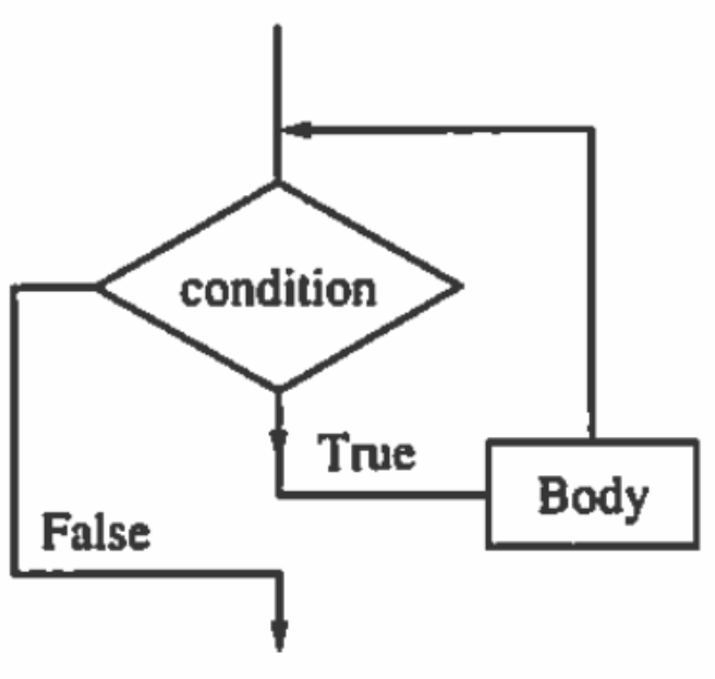
    clipboard_e5d947c72cb8066b9b83a86bf8423c77c.pngFigure \(\PageIndex{1}\): Flow diagram for a while loop

    Suppose you wanted to solve the equation \(f(x) = 0\text{.}\) The following initial assignment and loop could be employed.

    1. c = your first guess
    2. While f(c) != 0:
            c = another guess
    

    Listing \(\PageIndex{3}\)

    Note

    One must always guard against the possibility that the condition of a While loop will never become false. Such "infinite loops" are the bane of beginning programmers. The loop above could very well be such a situation, particularly if the equation has no solution, or if the variable takes on real values

    In cases where consecutive integer values are to be assigned to a variable, a different loop construction, a For loop, is often employed. For example, suppose we wanted to assign variable k each of the integer values from m to n and for each of these values perform some undefined steps. We could accomplish this with a While loop:

    1. k := m
    2. While k <= n:
        2.1 execute some steps
        2.2 k = k + l
    

    Listing \(\PageIndex{4}\)

    Alternatively, we can perform these steps with a For loop.

    For k = m to n:
        execute some  steps
    

    Listing \(\PageIndex{5}\)

    For loops such as this one have the advantage of being shorter than the equivalent While loop. The While loop construction has the advantage of being able to handle more different situations than the For loop.

    Exercises

    Exercise \(\PageIndex{1}\)

    What are the inputs and outputs of the algorithms listed in the first sentence of this section?

    Exercise \(\PageIndex{2}\)

    What is wrong with this algorithm?

    Input: a and b, integers
    Output: the value of c will be a - b
    (1) c = 0
    (2) While a > b:
            (2.1) a := a - l
            (2.2) c := c + l
    

    Listing \(\PageIndex{6}\)

    Answer

    The algorithm only works when a > b.

    Exercise \(\PageIndex{3}\)

    Describe, in words, what the following algorithm does:

    Input: k, a positive integer
    Output: s = ?
    (1) s = 0
    (2) While k > 0:
        (2.1) s = s + k
        (2.2) k = k - 1
    

    Listing \(\PageIndex{7}\)

    Exercise \(\PageIndex{4}\)

    Write While loops to replace the For loops in the following partial algorithms:

    1.  
      1. S = 0
      2. for k = 1 to 5: S = S + k^2
    2. The floor of a number is the greatest integer less than or equal to that number.
      1. m = a positive integer greater than 1
      2. B = floor(sqrt(m))
      3. for i = 2 to B: if i divides evenly into m, jump to step 5
      4. print "m is a prime" and exit
      5. print "m is composite" and exit

    Exercise \(\PageIndex{5}\)

    Describe in words what the following algorithm does:

    Input: n, a positive integer
    Output: k?
    (1) f= 0
    (2) k=n
    (3) While k is even:
        (3.1) f = f+ 1
        (3.2) k = k div 2
    

    Listing \(\PageIndex{8}\)

    Exercise \(\PageIndex{6}\)

    Fix the algorithm in Exercise \(\PageIndex{2}\).


    17.1.1: An Introduction to Algorithms is shared under a not declared license and was authored, remixed, and/or curated by LibreTexts.

    • Was this article helpful?