
14.1: Edge Coloring
- Page ID
- 60143

\( \newcommand{\vecs}[1]{\overset { \scriptstyle \rightharpoonup} {\mathbf{#1}} } \)
\( \newcommand{\vecd}[1]{\overset{-\!-\!\rightharpoonup}{\vphantom{a}\smash {#1}}} \)
\( \newcommand{\dsum}{\displaystyle\sum\limits} \)
\( \newcommand{\dint}{\displaystyle\int\limits} \)
\( \newcommand{\dlim}{\displaystyle\lim\limits} \)
\( \newcommand{\id}{\mathrm{id}}\) \( \newcommand{\Span}{\mathrm{span}}\)
( \newcommand{\kernel}{\mathrm{null}\,}\) \( \newcommand{\range}{\mathrm{range}\,}\)
\( \newcommand{\RealPart}{\mathrm{Re}}\) \( \newcommand{\ImaginaryPart}{\mathrm{Im}}\)
\( \newcommand{\Argument}{\mathrm{Arg}}\) \( \newcommand{\norm}[1]{\| #1 \|}\)
\( \newcommand{\inner}[2]{\langle #1, #2 \rangle}\)
\( \newcommand{\Span}{\mathrm{span}}\)
\( \newcommand{\id}{\mathrm{id}}\)
\( \newcommand{\Span}{\mathrm{span}}\)
\( \newcommand{\kernel}{\mathrm{null}\,}\)
\( \newcommand{\range}{\mathrm{range}\,}\)
\( \newcommand{\RealPart}{\mathrm{Re}}\)
\( \newcommand{\ImaginaryPart}{\mathrm{Im}}\)
\( \newcommand{\Argument}{\mathrm{Arg}}\)
\( \newcommand{\norm}[1]{\| #1 \|}\)
\( \newcommand{\inner}[2]{\langle #1, #2 \rangle}\)
\( \newcommand{\Span}{\mathrm{span}}\) \( \newcommand{\AA}{\unicode[.8,0]{x212B}}\)
\( \newcommand{\vectorA}[1]{\vec{#1}} % arrow\)
\( \newcommand{\vectorAt}[1]{\vec{\text{#1}}} % arrow\)
\( \newcommand{\vectorB}[1]{\overset { \scriptstyle \rightharpoonup} {\mathbf{#1}} } \)
\( \newcommand{\vectorC}[1]{\textbf{#1}} \)
\( \newcommand{\vectorD}[1]{\overrightarrow{#1}} \)
\( \newcommand{\vectorDt}[1]{\overrightarrow{\text{#1}}} \)
\( \newcommand{\vectE}[1]{\overset{-\!-\!\rightharpoonup}{\vphantom{a}\smash{\mathbf {#1}}}} \)
\( \newcommand{\vecs}[1]{\overset { \scriptstyle \rightharpoonup} {\mathbf{#1}} } \)
\(\newcommand{\longvect}{\overrightarrow}\)
\( \newcommand{\vecd}[1]{\overset{-\!-\!\rightharpoonup}{\vphantom{a}\smash {#1}}} \)
\(\newcommand{\avec}{\mathbf a}\) \(\newcommand{\bvec}{\mathbf b}\) \(\newcommand{\cvec}{\mathbf c}\) \(\newcommand{\dvec}{\mathbf d}\) \(\newcommand{\dtil}{\widetilde{\mathbf d}}\) \(\newcommand{\evec}{\mathbf e}\) \(\newcommand{\fvec}{\mathbf f}\) \(\newcommand{\nvec}{\mathbf n}\) \(\newcommand{\pvec}{\mathbf p}\) \(\newcommand{\qvec}{\mathbf q}\) \(\newcommand{\svec}{\mathbf s}\) \(\newcommand{\tvec}{\mathbf t}\) \(\newcommand{\uvec}{\mathbf u}\) \(\newcommand{\vvec}{\mathbf v}\) \(\newcommand{\wvec}{\mathbf w}\) \(\newcommand{\xvec}{\mathbf x}\) \(\newcommand{\yvec}{\mathbf y}\) \(\newcommand{\zvec}{\mathbf z}\) \(\newcommand{\rvec}{\mathbf r}\) \(\newcommand{\mvec}{\mathbf m}\) \(\newcommand{\zerovec}{\mathbf 0}\) \(\newcommand{\onevec}{\mathbf 1}\) \(\newcommand{\real}{\mathbb R}\) \(\newcommand{\twovec}[2]{\left[\begin{array}{r}#1 \\ #2 \end{array}\right]}\) \(\newcommand{\ctwovec}[2]{\left[\begin{array}{c}#1 \\ #2 \end{array}\right]}\) \(\newcommand{\threevec}[3]{\left[\begin{array}{r}#1 \\ #2 \\ #3 \end{array}\right]}\) \(\newcommand{\cthreevec}[3]{\left[\begin{array}{c}#1 \\ #2 \\ #3 \end{array}\right]}\) \(\newcommand{\fourvec}[4]{\left[\begin{array}{r}#1 \\ #2 \\ #3 \\ #4 \end{array}\right]}\) \(\newcommand{\cfourvec}[4]{\left[\begin{array}{c}#1 \\ #2 \\ #3 \\ #4 \end{array}\right]}\) \(\newcommand{\fivevec}[5]{\left[\begin{array}{r}#1 \\ #2 \\ #3 \\ #4 \\ #5 \\ \end{array}\right]}\) \(\newcommand{\cfivevec}[5]{\left[\begin{array}{c}#1 \\ #2 \\ #3 \\ #4 \\ #5 \\ \end{array}\right]}\) \(\newcommand{\mattwo}[4]{\left[\begin{array}{rr}#1 \amp #2 \\ #3 \amp #4 \\ \end{array}\right]}\) \(\newcommand{\laspan}[1]{\text{Span}\{#1\}}\) \(\newcommand{\bcal}{\cal B}\) \(\newcommand{\ccal}{\cal C}\) \(\newcommand{\scal}{\cal S}\) \(\newcommand{\wcal}{\cal W}\) \(\newcommand{\ecal}{\cal E}\) \(\newcommand{\coords}[2]{\left\{#1\right\}_{#2}}\) \(\newcommand{\gray}[1]{\color{gray}{#1}}\) \(\newcommand{\lgray}[1]{\color{lightgray}{#1}}\) \(\newcommand{\rank}{\operatorname{rank}}\) \(\newcommand{\row}{\text{Row}}\) \(\newcommand{\col}{\text{Col}}\) \(\renewcommand{\row}{\text{Row}}\) \(\newcommand{\nul}{\text{Nul}}\) \(\newcommand{\var}{\text{Var}}\) \(\newcommand{\corr}{\text{corr}}\) \(\newcommand{\len}[1]{\left|#1\right|}\) \(\newcommand{\bbar}{\overline{\bvec}}\) \(\newcommand{\bhat}{\widehat{\bvec}}\) \(\newcommand{\bperp}{\bvec^\perp}\) \(\newcommand{\xhat}{\widehat{\xvec}}\) \(\newcommand{\vhat}{\widehat{\vvec}}\) \(\newcommand{\uhat}{\widehat{\uvec}}\) \(\newcommand{\what}{\widehat{\wvec}}\) \(\newcommand{\Sighat}{\widehat{\Sigma}}\) \(\newcommand{\lt}{<}\) \(\newcommand{\gt}{>}\) \(\newcommand{\amp}{&}\) \(\definecolor{fillinmathshade}{gray}{0.9}\)Suppose you have been given the job of scheduling a round-robin tennis tournament with \(n\) players. One way to approach the problem is to model it as a graph: the vertices of the graph will represent the players, and the edges will represent the matches that need to be played. Since it is a round-robin tournament, every player must play every other player, so the graph will be complete. Creating the schedule amounts to assigning a time to each of the edges, representing the time at which that match is to be played.
Notice that there is a constraint. When you have assigned a time to a particular edge \(uv\), no other edge incident with either \(u\) or \(v\) can be assigned the same time, since this would mean that either player \(u\) or player \(v\) is supposed to play two games at once. Instead of writing times on each edge, we will choose a colour to represent each of the time slots, and colour the edges that are to be played at that time, with that colour.
Here is an example of a possible schedule for the tournament, when \(n = 7\).
Example \(\PageIndex{1}\)
The players are numbered from \(1\) through\(7\), and we will spread the tournament out over seven days. Games to be played on each day should have a different colour than the games on other days, but, because this text is printed in black-and-white, we will use some line patterns, instead of colours. Games to be played on Monday will be drawn as usual. Games to be played on Tuesday will be thin. Games to be played on Wednesday will be dotted. Games to be played on Thursday will be dashed. Games to be played on Friday will be thick. Games to be played on Saturday will be grey. Games to be played on Sunday will be thin and dashed.

This gives a schedule. For anyone who has trouble distinguishing the “colours” of the edges, the normal edges are \(12\), \(37\), and \(46\); the thin edges are \(13\), \(24\), and \(57\); the dotted edges are \(15\), \(26\), and \(34\); the dashed edges are \(17\), \(36\), and \(45\); the thick edges are \(23\), \(47\), and \(56\); the grey edges are \(14\), \(25\), and \(67\); and the thin dashed edges are \(16\), \(27\), and \(35\).
Definition: Proper \(k\)-Edge-Colouring
A proper \(k\)-edge-colouring of a graph \(G\) is a function that assigns to each edge of \(G\) one of \(k\) colours, such that edges that meet at an endvertex must be assigned different colours.
The constraint that edges of the same colour cannot meet at a vertex turns out to be a useful constraint in a number of contexts.
If the graph is large enough we are liable to run out of colours that can be easily distinguished (and we get tired of writing out the names of colours). The usual convention is to refer to each colour by a number (the first colour is colour \(1\), etc.) and to label the edges with the numbers rather than using colours.
Definition: \(k\)-Edge-Colourable
A graph \(G\) is \(k\)-edge-colourable if it admits a proper \(k\)-edge-colouring. The smallest integer \(k\) for which \(G\) is \(k\)-edge-colourable is called the edge chromatic number, or chromatic index of \(G\).
Notation
The chromatic index of \(G\) is denoted by \(χ'(G)\), or simply by \(χ'\) if the context is unambiguous.
Here is an easy observation:
Proposition \(\PageIndex{1}\)
For any graph \(G\), \(χ'(G) ≥ ∆(G)\).
- Proof
-
Recall that \(∆(G)\) denotes the maximum value of \(d(v)\) over all vertices \(v\) of \(G\). So there is some vertex \(v\) of \(G\) such that \(d(v) = ∆(G)\). In any proper edge-colouring, the \(d(v)\) edges that are incident with \(v\), must all be assigned different colours. Thus, any proper edge-colouring must have at least \(d(v) = ∆(G)\) distinct colours. This means \(χ'(G) ≥ ∆(G)\).
Example \(\PageIndex{2}\)
The colouring given in Example 14.1.1 shows that \(χ'(K_7) ≤ 7\), since we were able to properly edge-colour \(K_7\) using seven colours.
To show that we cannot colour \(K_7\) with fewer than \(7\) colours, notice that because each of the \(7\) vertices can only be incident with one edge of a given colour, there cannot be more than \(3\) edges coloured with any given colour (\(3\) edges are already incident with \(6\) of the \(7\) vertices, and a fourth edge would have to be incident with two others).
We know that \(K_7\) has \(\binom{7}{2} = 21\) edges, so if at most \(3\) edges can be coloured with any given colour, we will require at least \(7\) colours to properly edge-colour \(K_7\). Thus \(χ'(K_7) ≥ 7\).
Thus, we have shown that \(χ'(K_7) = 7\).
This shows that \(χ'(K_7) = 7 > ∆(K_7) = 6\), so it is not always possible to achieve equality in the bound given by Proposition 14.1.1. Our next example shows that it is sometimes possible to achieve equality in that bound
Example \(\PageIndex{3}\)
Here is a proper \(5\)-edge-colouring of \(K_6\):

In case the edge colours are difficult to distinguish, the thick edges are \(12\), \(36\), and \(45\); the thin edges are \(13\), \(24\), and \(56\); the dotted edges are \(14\), \(26\), and \(35\); the dashed edges are \(15\), \(23\), and \(46\); and the grey edges are \(16\), \(25\), and \(34\). This shows that \(χ'(K_6) ≤ 5\). Since the valency of every vertex of \(K_6\) is \(5\), Proposition 14.1.1 implies that \(χ'(K_6) ≥ 5\). Putting these together, we see that \(χ'(K_6) = ∆(K_6) = 5\), so equality in the bound of Proposition 14.1.1 is achieved by \(K_6\).
The following rather remarkable result was proven by Vadim Vizing in \(1964\):
Theorem \(\PageIndex{1}\): Vizing's Theorem
For any simple graph \(G\), \(χ'(G) ∈ \{∆(G), ∆(G) + 1\}\).
- Proof
-
We will not go over the proof of this theorem.
Definition: Class One Graph and Class Two Graph
If \(χ'(G) = ∆(G)\) then \(G\) is said to be a class one graph, and if \(χ'(G) = ∆(G) + 1\) then \(G\) is said to be a class two graph.
To date, graphs have not been completely classified according to which graphs are class one and which are class two, but it has been proven that “almost every” graph is of class one. Technically, this means that if you choose a random graph out of all of the graphs on at most \(n\) vertices, the probability that you will choose a class two graph approaches \(0\) as \(n\) approaches infinity.
There are, however, infinitely many class two graphs; the same argument we used to show that \(χ'(K_7) ≥ 7\) can also be used to prove that \(χ'(K_{2n+1}) = 2n + 1\) for any positive integer \(n\), since the number of edges is
\[\dfrac{(2n + 1)(2n)}{2} = n(2n + 1)\]
and each colour can only be used to colour \(n\) of the edges. Since \(∆(K_{2n+1}) = 2n\), this shows that \(K_{2n+1}\) is class two.
Large families of graphs have been shown to be class one graphs. We will devote most of the rest of this section to proving that all of the graphs in one particular family are class one. First, we need to define the family.
Definition: Bipartition
A graph is bipartite if its vertices can be partitioned into two sets \(V_1\) and \(V_2\), such that every edge of the graph has one of its endvertices in \(V_1\), and the other in \(V_2\). The sets \(V_1\) and \(V_2\) form a bipartition of the graph.
Example \(\PageIndex{4}\)
The following graphs are bipartite. Every edge has one endvertex on the left side, and one on the right.

The graph \(K_n\) is not bipartite if \(n ≥ 3\). The first vertex may as well go into \(V_1\); the second vertex is adjacent to it, so must go into \(V_2\); but the third vertex is adjacent to both, so cannot go into either \(V_1\) or \(V_2\).
Although the following class of bipartite graphs will not be used in this chapter, they are an important class of bipartite graphs that will come up again later.
Definition: Complete Bipartite Graph
The complete bipartite graph, \(K_{m,n}\), is the bipartite graph on \(m + n\) vertices with as many edges as possible subject to the constraint that it has a bipartition into sets of cardinality \(m\) and \(n\). That is, it has every edge between the two sets of the bipartition.
Before proving that all bipartite graphs are class one, we need to understand the structure of bipartite graphs a bit better. Here is an important theorem.
Theorem \(\PageIndex{2}\)
A graph \(G\) is bipartite if and only if \(G\) contains no cycle of odd length.
- Proof
-
This is an if and only if statement, so we have two implications to prove.
\((⇒)\) We prove the contrapositive, that if \(G\) contains a cycle of odd length, then \(G\) cannot be bipartite.
Let
\[(v_1, v_2, . . . , v_{2k+1}, v_1)\]
be a cycle of odd length in \(G\). We try to establish a bipartition \(V_1\) and \(V_2\) for \(G\). Without loss of generality, we may assume that \(v_1 ∈ V_1\). Then we must have \(v_2 ∈ V_2\) since \(v_2 ∼ v_1\). Continuing in this fashion around the cycle, we see that for every \(1 ≤ i ≤ k\), we have \(v_{2i+1} ∈ V_1\) and \(v_{2i} ∈ V_2\). In particular, \(v_{2k+1} ∈ V_1\), but \(v_1 ∈ V_1\) and \(v_1 ∼ v_{2k+1}\), contradicting the fact that every edge must have one of its endvertices in \(V_2\). Thus, \(G\) is not bipartite.
\((⇐)\) Let \(G\) be a graph that is not bipartite. We must show that there is an odd cycle in \(G\).
If every connected component of \(G\) is bipartite, then \(G\) is bipartite (choose one set of the bipartition from each connected component; let \(V_1\) be the union of these, and \(V_2\) the set of all other vertices of \(G\); this is a bipartition for \(G\)). Thus there is at least one connected component of \(G\) that is not bipartite.
Pick any vertex \(u\) from a non-bipartite connected component of \(G\), and assign it to \(V_1\). Place all of its neighbours in \(V_2\). Place all of their neighbours into \(V_1\). Repeat this process, at each step putting all of the neighbours of every vertex of \(V_1\) into \(V_2\), and then all of the neighbours of every vertex of \(V_2\) into \(V_1\).
Since this component is not bipartite, at some point we must run into the situation that we place a vertex \(v\) into \(V_j\), but a neighbour \(u_1\) of \(v\) is also in \(V_j\) (for some \(j ∈ \{1, 2\}\)). By our construction of \(V_1\) and \(V_2\), there must be a walk from \(u_1\) to \(v\) that alternates between vertices in \(V_j\) and vertices in \(V_{3−j}\). By Proposition 12.3.1, there must in fact be a path from \(u_1\) to \(v\) that alternates between vertices in \(V_j\) and vertices in \(V_{3−j}\). Since the path alternates between the two sets but begins and ends in \(V_j\), it has even length. Therefore, adding \(u_1\) to the end of this path yields a cycle of odd length in \(\)G.
In order to prove that bipartite graphs are class one, we require a lemma.
Lemma \(\PageIndex{1}\)
Let \(G\) be a connected graph that is not a cycle of odd length. Then \(G\) the edges of \(G\) can be \(2\)-coloured so that edges of both colours are incident with every non-leaf vertex. (Note: this will probably not be a proper \(2\)-edge-colouring of \(G\).)
- Proof
-
We first consider the case where every vertex of \(G\) has even valency.
Choose a vertex \(v\) of \(G\) subject to the constraint that if any vertex of \(G\) has valency greater than \(2\), then \(v\) is such a vertex. Since every vertex of \(G\) has even valency, we can find an Euler tour of \(G\) that begins and ends at \(v\). Alternate edge colours around this tour. Clearly, every vertex that is visited in the middle of the tour (that is, every vertex except possibly \(v\)) must be incident with edges of both colours, since whichever colour is given to the edge we travel to reach that vertex, the other colour will be given to the edge we travel when leaving that vertex. If any vertex of \(G\) has valency greater than \(2\), then by our choice of \(v\), the valency of \(v\) must be greater than \(2\), so \(v\) is visited in the middle of the tour, and this colouring has the desired property. If every vertex of \(G\) has valency \(2\), then since \(G\) is connected, \(G\) must be a cycle (see Exercise 12.3.1(4). Since \(G\) is not a cycle of odd length (by hypothesis), \(G\) must be a cycle of even length. Therefore the number of edges of \(G\) is even, so the tour will begin and end with edges of opposite colours, both of which are incident with \(v\). Again we see that this colouring has the desired property.
Suppose now that \(G\) has at least one vertex of odd valency.
Create a new vertex, \(u\), and add edges between \(u\) and every vertex of \(G\) that has odd valency. All of the vertices of \(G\) will have even valency in this new graph, and by the corollary to Euler’s handshaking lemma, \(u\) must also have even valency, so this graph has an Euler tour; in fact, we can find an Euler tour that begins with the vertex \(u\). Alternate edge colours around this tour. Delete \(u\) (and its incident edges) but retain the colours on the edge of \(G\). We claim that this colouring will have the desired property. If a vertex \(v\) has even valency in \(G\), it must be visited in the middle of the tour and the edges we travel on to reach \(v\) and to leave \(v\) will have different colours. Neither of these edges is incident with \(u\), so both are in \(G\). If a vertex \(v\) has valency \(1\) in \(G\), then \(v\) is a leaf and the colour of its incident edge doesn’t matter. If a vertex \(v\) has odd valency at least \(3\) in \(G\), then \(v\) is visited at least twice in the middle of the tour. Only one of these visits can involve the edge \(uv\), so during any other visit, the edges we travel on to reach \(v\) and to leave \(v\) will have different colours. Neither of these edges is incident with \(u\), so both are in \(G\). Thus, this colouring has the desired property.
Notation
Given a (not necessarily proper) edge-colouring \(\mathcal{C}\), we use \(c(v)\) to denote the number of distinct colours that have be used on edges that are incident with \(v\). Clearly, \(c(v) ≤ d(v)\).
Definition: Improvement and Optimal
An edge colouring \(\mathcal{C}'\) is an improvement on an edge colouring \(\mathcal{C}\) if it uses the same colours as \(\mathcal{C}\), but \(\sum_{v∈V} c'(v) > \sum_{v∈V} c(v)\).
An edge colouring is optimal if no improvement is possible.
Notice that since \(c(v) ≤ d(v)\) for every \(v ∈ V\), if
\[\sum_{v∈V}c(v) = \sum_{v∈V}d(v) \]
then we must have \(c(v) = d(v)\) for every \(v ∈ V\). This is precisely equivalent to the definition of a proper colouring.
At last, we are ready to prove that bipartite graphs are class one.
Theorem \(\PageIndex{3}\)
If \(G\) is bipartite, then \(χ'(G) = ∆(G)\).
- Proof
-
Let \(G\) be a bipartite graph. Towards a contradiction, suppose that \(χ'(G) > ∆(G)\).
Let \(\mathcal{C}\) be an optimal \(∆(G)\)-edge-colouring of \(G\). By assumption, \(\mathcal{C}\) will not be a proper edge colouring, so there must be some vertex \(u\) such that \(c(u) < d(u)\). By the Pigeonhole Principle, some colour \(j\) must be used to colour at least two of the edges incident with \(u\), and since there are \(∆(G) ≥ d(u)\) colours in total and only \(c(u)\) are used on edges incident with \(u\), there must be some colour \(i\) that is not used to colour any edge incident with \(u\).
Consider only the edges of \(G\) that have been coloured with either \(i\) or \(j\) in the colouring \(\mathcal{C}\). Since \(G\) is bipartite, these edges cannot include an odd cycle. We apply Lemma 14.1.1 to each connected component formed by these edges to re-colour these edges. Our re-colouring will use only colours \(i\) and \(j\), and if a vertex \(v\) was incident to at least two edges coloured with either \(i\) or \(j\) in \(\mathcal{C}\), then under the re-colouring, \(v\) will be incident with at least one edge coloured with \(i\) and at least one edge coloured with \(j\). Leave all of the other edge colours alone, and call this new colouring \(\mathcal{C}'\).
We claim that \(\mathcal{C}'\) is an improvement on \(\mathcal{C}\). Any vertex \(v\) that had at most one incident edge coloured with either \(i\) or \(j\) under \(\mathcal{C}\), will still have exactly the same colours except that the edge coloured \(i\) or \(j\) might have switched its colour to the other of \(i\) and \(j\). In any case, we will have \(c'(v) = c(v)\). Any vertex \(v\) that had at least two incident edges coloured with either \(i\) or \(j\) under \(\mathcal{C}\), will still have all of the same colours except that it will now have incident edges coloured with both \(i\) and \(j\), so \(c'(v) ≥ c(v)\). Furthermore, we have \(c'(u) > c(u)\) since the edges incident with \(u\) now include edges coloured with both \(i\) and \(j\), where before there were only edges coloured with \(j\). Thus,
\[\sum_{v∈V}c'(v) = \sum_{v∈V}c(v) \]
so \(\mathcal{C}'\) is an improvement on \(\mathcal{C}\), as claimed.
We have contradicted our assumption that \(\mathcal{C}\) is an optimal \(∆(G)\)-edge-colouring. This contradiction serves to prove that \(χ'(G) = ∆(G)\).
Exercise \(\PageIndex{1}\)
1) Prove that every tree is a class one graph.
2) Prove that every cycle of odd length is a class two graph.
3) Find a graph that contains a cycle of odd length, but is a class one graph.
4) For each of the following graphs, find the edge-chromatic number, determine whether the graph is class one or class two, and find a proper edge-colouring that uses the smallest possible number of colours.
(a) The two graphs in Exercise 13.2.1(2).
(b) The two graphs in Example 14.1.4.
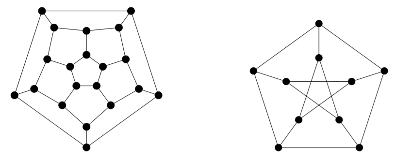
(c) The skeleton of a dodecahedron (the leftmost of the two graphs drawn below).
(d) The Petersen graph (the rightmost of the two graphs drawn below). You may assume, without proof, that the Petersen graph is class two.
5) Find a systematic approach to colouring the edges of complete graphs that demonstrates that \(χ'(K_{2n−1}) = χ'(K_{2n}) = 2n − 1\).
6) Find a systematic approach to colouring the edges of complete bipartite graphs that demonstrates that \(χ'(K_{m,n}) = ∆(K_{m,n}) = \max\{m, n\}\).
Exercise \(\PageIndex{2}\)
The following exercises illustrate some of the connections between Hamilton cycles and edge-colouring.
1) Definition. A graph is said to be Hamilton-connected if there is a Hamilton path from each vertex in the graph to each of the other vertices in the graph. Prove that if \(G\) is bipartite and has at least \(3\) vertices, then \(G\) is not Hamiltonconnected.
[Hint: Prove this by contradiction. Consider the length of a Hamilton path and where it can end.]
2) Suppose that \(G\) is a bipartite graph with \(V_1\) and \(V_2\) forming a bipartition. Show that if \(|V1| \neq |V2|\) then \(G\) has no Hamilton cycle.
3) Prove that if every vertex of \(G\) has valency \(3\), and \(G\) has a Hamilton cycle, then \(G\) is class one.
[Hint: Use the corollary to Euler’s handshaking lemma, and find a way to assign colours to the edges of the Hamilton cycle.]