14.3: Vertex Colouring

Last updated
Save as PDF

Page ID: 60145

Joy Morris
University of Lethbridge

$ \newcommand{\vecs}[1]{\overset { \scriptstyle \rightharpoonup} {\mathbf{#1}} } $ $ \newcommand{\vecd}[1]{\overset{-\!-\!\rightharpoonup}{\vphantom{a}\smash {#1}}} $$\newcommand{\id}{\mathrm{id}}$ $ \newcommand{\Span}{\mathrm{span}}$ $ \newcommand{\kernel}{\mathrm{null}\,}$ $ \newcommand{\range}{\mathrm{range}\,}$ $ \newcommand{\RealPart}{\mathrm{Re}}$ $ \newcommand{\ImaginaryPart}{\mathrm{Im}}$ $ \newcommand{\Argument}{\mathrm{Arg}}$ $ \newcommand{\norm}[1]{\| #1 \|}$ $ \newcommand{\inner}[2]{\langle #1, #2 \rangle}$ $ \newcommand{\Span}{\mathrm{span}}$ $\newcommand{\id}{\mathrm{id}}$ $ \newcommand{\Span}{\mathrm{span}}$ $ \newcommand{\kernel}{\mathrm{null}\,}$ $ \newcommand{\range}{\mathrm{range}\,}$ $ \newcommand{\RealPart}{\mathrm{Re}}$ $ \newcommand{\ImaginaryPart}{\mathrm{Im}}$ $ \newcommand{\Argument}{\mathrm{Arg}}$ $ \newcommand{\norm}[1]{\| #1 \|}$ $ \newcommand{\inner}[2]{\langle #1, #2 \rangle}$ $ \newcommand{\Span}{\mathrm{span}}$$\newcommand{\AA}{\unicode[.8,0]{x212B}}$

Suppose you have been given the task of assigning broadcast frequencies to transmission towers. You have been given a list of frequencies that you are permitted to assign. There is a constraint: towers that are too close together cannot be assigned the same frequency, since they would interfere with each other.

One way to approach this problem is to model it as a graph. The vertices of the graph will represent the towers, and the edges will represent towers that can interfere with each other. Your job is to assign a frequency to each of the vertices. Instead of writing a frequency on each vertex, we will choose a colour to represent that frequency, and use that colour to colour the vertices to which you assign that frequency.

Here is an example of this.

Example $\PageIndex{1}$

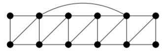
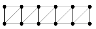
This graph represents the towers and their interference patterns.

$clipboard_e8d83cbeaf0952764c72eb7a53422df4e.png$

This represents a possible assignment of $4$ colours to the vertices. The colour of each vertex (red, green, blue, or yellow) is indicated by writing the first letter of the colour’s name on the vertex).

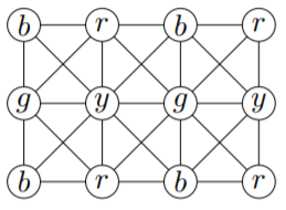
$clipboard_eeb77390fd8f60f767aa564d4f7a2f92d.png$

Notice that this colouring obeys the constraint that interfering towers are not assigned the same frequencies.

Definition: Proper $k$-Vertex-Colouring

A proper $k$-vertex-colouring (or just $k$-colouring) of a graph $G$ is a function that assigns to each vertex of $G$ one of $k$ colours, such that adjacent vertices must be assigned different colours.

As with edge-colouring, the constraint that adjacent vertices receive different colours turns out to be a useful constraint that arises in many contexts. We often represent the $k$ colours by the numbers $1, . . . , k$, and label the vertices with the appropriate numbers rather than colouring them.

Definition: $k$-Colourable

A graph $G$ is $k$-colourable if it admits a proper $k$-(vertex-)colouring. The smallest integer $k$ for which $G$ is $k$-colourable is called the chromatic number of $G$.

Notation

The chromatic number of $G$ is denoted by $χ(G)$, or simply by $χ$ if the context is unambiguous.

We leave the proof of the following as an exercise (see Exercise 14.3.1(2)).

Proposition $\PageIndex{1}$

For every $n ≥ 1$, $χ(K_n) = n$.

Example $\PageIndex{2}$

Prove that for a graph $G$, $χ(G) = 2$ if and only if $G$ is a bipartite graph that has at least one edge.

Solution

$(⇒)$ Suppose that $χ(G) = 2$. Take a proper $2$-colouring of $G$ with colours $1$ and $2$. Let $V_1$ denote the set of vertices of colour $1$, and let $V_2$ denote the set of vertices of colour $2$. Since the colouring is proper, there are no edges both of whose endvertices are in $V_1$ (as these would be adjacent vertices both coloured with colour $1$). Similarly, there are no edges both of whose endvertices are in $V_2$. Thus, the sets $V_1$ and $V_2$ form a bipartition of $G$, so $G$ is bipartite. Since $2$ colours were required to properly colour $G$, $G$ must have at least one edge.

$(⇐)$ Suppose that $G$ is bipartite, and that $V_1$ and $V_2$ form a bipartition of $G$. Colour the vertices in $V_1$ with colour $1$, and colour the vertices of $V_2$ with colour $2$. By the definition of a bipartition, no pair of adjacent vertices can have been assigned the same colour. Thus, this is a proper $2$-colouring of $G$, so $χ(G) ≤ 2$. Since $G$ has at least one edge, the endpoints of that edge must be assigned different colours, so $χ(G) ≥ 2$. Thus $χ(G) = 2$.

Example $\PageIndex{3}$

Show that for any $n ≥ 1$, $χ(C_{2n+1}) = 3$.

Solution

Since this graph has an edge whose endvertices must be assigned different colours, we see that $χ(C_{2n+1}) ≥ 2$. Since a cycle of odd length is not bipartite (see Theorem 14.1.2), Example 14.3.2 shows that $χ(C_{2n+1}) \neq 2$, so $χ(C_{2n+1}) ≥ 3$. Let the cycle be $(u_1, u_2, . . . , u_{2n+1}, u_1)$. Since the only edges in the graph are between consecutive vertices in this list, if we assign colour $1$ to $u_1$, colour $2$ to $u_{2i}$ for $1 ≤ i ≤ n$, and colour $3$ to $u_{2i+1}$ for $1 ≤ i ≤ n$, this will be a proper $3$-colouring. Thus, $χ(C_{2n+1}) = 3$.

Definition: $k$-Critical

A graph $G$ is k-critical if $χ(G) = k$, but for every proper subgraph $H$ of $G$, $χ(H) < χ(G)$.

Proposition $\PageIndex{2}$

Any $k$-critical graph is connected.

Proof

Towards a contradiction, suppose that $G$ is a disconnected $k$-critical graph, and let $G_1$ and $G_2$ be (nonempty) subgraphs of $G$ such that every vertex of $G$ is in either $G_1$ or $G_2$, and there is no edge from any vertex in $G_1$ to any vertex in $G_2$. By the definition of $k$-critical, $χ(G_1) < χ(G)$ and $χ(G_2) < χ(G)$. But if we colour $G_1$ with $χ(G_1)$ colours and $G_2$ with $χ(G_2)$ colours, since there is no edge from any vertex of $G_1$ to any vertex of $G_2$, this produces a proper colouring of $G$ with

\[\max(χ(G_1), χ(G_2)) < χ(G)\]

colours. This contradiction serves to prove that every $k$-critical graph is connected.

Theorem $\PageIndex{1}$

If $G$ is $k$-critical, then $δ(G) ≥ k − 1$.

Proof: Towards a contradiction, suppose that $G$ is $k$-critical and has a vertex $v$ of valency at most $k −2$. By the definition of $k$-critical, $G \setminus \{v\}$ must be $(k −1)$-colourable. Now, since $v$ has no more than $k − 2$ neighbours, its neighbours can be assigned at most $k − 2$ distinct colours in this colouring. Therefore, amongst the colours used in the $(k − 1)$-colouring of $G \setminus \{v\}$, there must be a colour that is not assigned to any of the neighbours of $v$. If we assign this colour to $v$, the result is a proper $(k − 1)$-colouring of $G$, contradicting $χ(G) = k$. This contradiction serves to prove that every $k$-critical graph has minimum valency at least $k − 1$.

Corollary $\PageIndex{1}$

For any graph $G$, $χ(G) ≤ ∆(G) + 1$.

Proof

Let $G$ be an arbitrary graph. By deleting as many edges and vertices as it is possible to delete without reducing the chromatic number (we can never increase the chromatic number by deleting vertices or edges, see Exercise 14.3.1(1)), we see that $G$ must have a subgraph $H$ that is $χ(G)$-critical. By Theorem 14.3.1, we see that

\[δ(H) ≥ χ(G) − 1.\]

Thus, every vertex of $H$ has valency at least $χ(G) − 1$, so in $G$, these same vertices still have valency at least $χ(G) − 1$. For any such vertex $v$, we have

\[∆(G) ≥ d(v) ≥ χ(G) − 1,\]

so $χ(G) ≤ ∆(G) + 1$.

We have already seen two families of graphs for which this bound is attained: for complete graphs, we have

\[∆(K_n) + 1 = (n − 1) + 1 = n = χ(K_n)\]

(see Proposition 14.3.1); and for cycles of odd length, we have

\[∆(C_{2n+1}) + 1 = 2 + 1 = 3 = χ(C_{2n+1})\]

(see Example 14.3.3). In fact, Brooks proved in 1941 that these are the only connected graphs for which this bound is obtained.

Theorem $\PageIndex{2}$: Brook's Theorem

If $G$ is connected and for every $n ≥ 1$, $G \ncong C_{2n+1}$ and $G \ncong K_n$, then $χ(G) ≤ ∆(G)$.

Proof: We will not include the proof of this result in this course. This theorem does allow us to determine the chromatic number of some graphs with very little work.

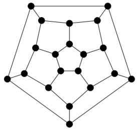
Example $\PageIndex{4}$

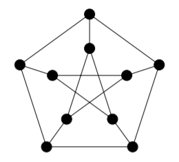
The following very famous graph is called the Petersen graph. It is an exceptional graph in many ways, so when mathematicians are trying to come up with a proof or a counterexample in graph theory, it is often one of the first examples they will check. Find its chromatic number.

$clipboard_ec0db06837b987f121c2d381120de1ad0.png$

Solution

We have $∆ = 3$, and since this graph is neither a complete graph nor a cycle of odd length, by Brooks’ Theorem this shows that $χ ≤ 3$. We can find a cycle of length $5$ around the outer edge of the graph, so this graph is not bipartite but has an edge. Therefore (by Example 14.3.2), $χ > 2$. Hence $χ = 3$.

Exercise $\PageIndex{1}$

1) Prove that if $H$ is a subgraph of $G$ then $χ(G) ≥ χ(H)$.

2) Prove Proposition 14.3.1 by induction.

3) Prove Corollary 14.3.1 by induction for every graph on at least one vertex.

4) For each $i$, $j ∈ \{4, 5, 6\}$, suppose you are given a graph $G$ that contains a subgraph isomorphic to $K_i$ and no vertex has more than $j$ neighbours. What (if anything) can you say about $χ(G)$? Can you say more if you know that $G$ is connected and is neither a complete graph nor a cycle of odd length?

Exercise $\PageIndex{2}$

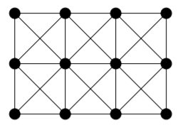
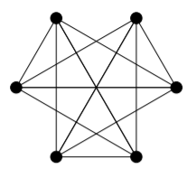
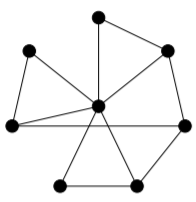
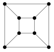
For each of the following graphs, determine its chromatic number by using theoretical arguments to provide a lower bound, and then producing a colouring that meets the bound. Do the same for the edge-chromatic number.

1) $clipboard_ebb943566c31d45fb179a3e11db027e16.png$