2.9: Applications

In this section we will describe several applications leading to systems of differential equations. In keeping with common practice in areas like physics, we will denote differentiation with respect to time as

\[\dot{x}=\dfrac{d x}{d t} \nonumber \]

We will look mostly at linear models and later modify some of these models to include nonlinear terms.

2.9.1 Spring-Mass Systems

There are many problems in physics that result in systems of equations. This is because the most basic law of physics is given by Newton's Second Law, which states that if a body experiences a net force, it will accelerate. In particular, the net force is proportional to the acceleration with a proportionality constant called the mass, \(m\). This is summarized as

\[\sum \mathbf{F}=m \mathbf{a} \nonumber \]

Since \(\mathbf{a}=\ddot{\mathbf{x}}\), Newton's Second Law is mathematically a system of second order differential equations for three dimensional problems, or one second order differential equation for one dimensional problems. If there are several masses, then we would naturally end up with systems no matter how many dimensions are involved.

A standard problem encountered in a first course in differential equations is that of a single block on a spring as shown in Figure 2.18. The net force in this case is the restoring force of the spring given by Hooke's Law,

\(F_{s}=-k x\),

where \(k>0\) is the spring constant. Here \(x\) is the elongation of the spring, or the displacement of the block from equilibrium. When \(x\) is positive, the spring force is negative and when \(x\) is negative the spring force is positive. We have depicted a horizontal system sitting on a frictionless surface.

A similar model can be provided for vertically oriented springs. Place the block on a vertically hanging spring. It comes to equilibrium, stretching the spring by \(\ell_{0}\). Newton's Second Law gives

\[-m g+k \ell_{0}=0 \nonumber \]

Now, pulling the mass further by \(x_{0}\), and releasing it, the mass begins to oscillate. Letting \(x\) be the displacement from the new equilibrium, Newton's Second Law now gives \(m \ddot{x}=-m g+k\left(\ell_{0}-x\right)=-k x\).

In both examples (a horizontally or vetically oscillating mass) Newton's Second Law of motion reults in the differential equation

\[m \ddot{x}+k x=0 \label{2.79} \]

This is the equation for simple harmonic motion which we have already encountered in Chapter 1.

Figure 2.18. Spring-Mass system.

This second order equation can be written as a system of two first order equations.

\[\begin{aligned}
&x^{\prime}=y \\
&y^{\prime}=-\dfrac{k}{m} x .
\end{aligned} \label{2.80} \]

The coefficient matrix for this system is

\(A=\left(\begin{array}{cc}
0 & 1 \\
-\omega^{2} & 0
\end{array}\right)\),

where \(\omega^{2}=\dfrac{k}{m}\). The eigenvalues of this system are \(\lambda=\pm i \omega\) and the solutions are simple sines and cosines,

\[\begin{aligned}
x(t) &=c_{1} \cos \omega t+c_{2} \sin \omega t \\
y(t) &=\omega\left(-c_{1} \sin \omega t+c_{2} \cos \omega t\right)
\end{aligned} \label{2.81} \]

We further note that \(\omega\) is called the angular frequency of oscillation and is given in \(\mathrm{rad} / \mathrm{s}\). The frequency of oscillation is

\[f=\dfrac{\omega}{2 \pi} \nonumber \]

It typically has units of \(\mathrm{s}^{-1}, \mathrm{cps}\), or \(\mathrm{Hz}\). The multiplicative inverse has units of time and is called the period,

\[T=\dfrac{1}{f} \nonumber \]

Thus, the period of oscillation for a mass \(m\) on a spring with spring constant \(k\) is given by

\[T=2 \pi \sqrt{\dfrac{m}{k}} \label{2.82} \]

Of course, we did not need to convert the last problem into a system. In fact, we had seen this equation in Chapter 1. However, when one considers

Figure 2.19. Spring-Mass system for two masses and two springs.

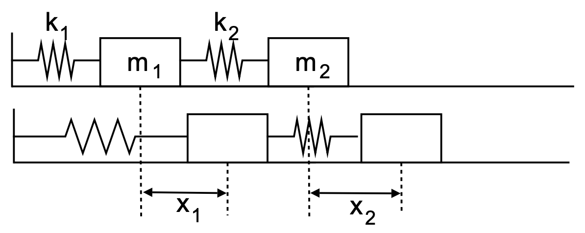
more complicated spring-mass systems, systems of differential equations occur naturally. Consider two blocks attached with two springs as shown in Figure 2.19. In this case we apply Newton’s second law for each block.

First, consider the forces acting on the first block. The first spring is stretched by \(x_{1}\). This gives a force of \(F_{1}=-k_{1} x_{1}\). The second spring may also exert a force on the block depending if it is stretched, or not. If both blocks are displaced by the same amount, then the spring is not displaced. So, the amount by which the spring is displaced depends on the relative displacements of the two masses. This results in a second force of \(F_{2}=k_{2}\left(x_{2}-x_{1}\right)\).

There is only one spring connected to mass two. Again the force depends on the relative displacement of the masses. It is just oppositely directed to the force which mass one feels from this spring.

Combining these forces and using Newton's Second Law for both masses, we have the system of second order differential equations

\[\begin{aligned}
&m_{1} \ddot{x}_{1}=-k_{1} x_{1}+k_{2}\left(x_{2}-x_{1}\right) \\
&m_{2} \ddot{x}_{2}=-k_{2}\left(x_{2}-x_{1}\right) .
\end{aligned} \label{2.83} \]

One can rewrite this system of two second order equations as a system of four first order equations. This is done by introducing two new variables \(x_{3}=\dot{x}_{1}\) and \(x_{4}=\dot{x}_{2}\). Note that these physically are the velocities of the two blocks.
The resulting system of first order equations is given as

\[\begin{aligned}
&\dot{x}_{1}=x_{3} \\
&\dot{x}_{2}=x_{4} \\
&\dot{x}_{3}=-\dfrac{k_{1}}{m_{1}} x_{1}+\dfrac{k_{2}}{m_{1}}\left(x_{2}-x_{1}\right) \\
&\dot{x}_{4}=-\dfrac{k_{2}}{m_{2}}\left(x_{2}-x_{1}\right)
\end{aligned} \label{2.84} \]

We can write our new system in matrix form as

\[\left(\begin{array}{l}
\dot{x}_{1} \\
\dot{x}_{2} \\
\dot{x}_{3} \\
\dot{x}_{4}
\end{array}\right)=\left(\begin{array}{cccc}
0 & 0 & 1 & 0 \\
0 & 0 & 0 & 1 \\
-\dfrac{k_{1}+k_{2}}{m_{1}} & \dfrac{k_{2}}{m_{1}} & 0 & 0 \\
\dfrac{k_{2}}{m_{2}} & -\dfrac{k_{2}}{m_{2}} & 0 & 0
\end{array}\right)\left(\begin{array}{l}
x_{1} \\
x_{2} \\
x_{3} \\
x_{4}
\end{array}\right) \label{2.85} \]

2.9.2 Electrical Circuits

Another problem often encountered in a first year physics class is that of an LRC series circuit. This circuit is pictured in Figure 2.20. The resistor is a circuit element satisfying Ohm's Law. The capacitor is a device that stores electrical energy and an inductor, or coil, stores magnetic energy.

The physics for this problem stems from Kirchoff's Rules for circuits. Since there is only one loop, we will only need Kirchoff's Loop Rule. Namely, the sum of the drops in electric potential are set equal to the rises in electric potential. The potential drops across each circuit element are given by

1. Resistor: \(V_{R}=I R\).
2. Capacitor: \(V_{C}=\dfrac{q}{C}\).
3. Inductor: \(V_{L}=L \dfrac{d I}{d t}\).

Figure 2.20. Series LRC Circuit.

Adding these potential drops and setting the sum equal to the voltage supplied by the voltage source, \(V (t)\), we obtain

\[I R+\dfrac{q}{C}+L \dfrac{d I}{d t}=V(t) \nonumber \]

Furthermore, we recall that the current is defined as \(I=\dfrac{d q}{d t}\). where \(q\) is the charge in the circuit. Since both \(q\) and \(I\) are unknown, we can replace the current by its expression in terms of the charge to obtain

\[L \ddot{q}+R \dot{q}+\dfrac{1}{C} q=V(t) \label{2.86} \]

This is a second order differential equation for \(q(t)\). One can set up a system of equations and proceed to solve them. However, this is a constant coefficient differential equation and can also be solved using the methods in Chapter 1.

In the next examples we will look at special cases that arise for the series LRC circuit equation. These include \(RC\) circuits, solvable by first order methods and \(LC\) circuits, leading to oscillatory behavior.

Example 2.19. RC Circuits

We first consider the case of an RC circuit in which there is no inductor.

Also, we will consider what happens when one charges a capacitor with a DC battery \(\left(V(t)=V_{0}\right)\) and when one discharges a charged capacitor \((V(t)=0)\).
For charging a capacitor, we have the initial value problem

\[R \dfrac{d q}{d t}+\dfrac{q}{C}=V_{0}, \quad q(0)=0 \label{2.87} \]

This equation is an example of a linear first order equation for \(q(t)\). However, we can also rewrite this equation and solve it as a separable equation, since \(V_{0}\) is a constant. We will do the former only as another example of finding the integrating factor.
We first write the equation in standard form:

\[\dfrac{d q}{d t}+\dfrac{q}{R C}=\dfrac{V_{0}}{R} \label{2.88} \]

The integrating factor is then

\[\mu(t)=e^{\int \dfrac{d t}{R C}}=e^{t / R C} \nonumber \]

Thus,

\[\dfrac{d}{d t}\left(q e^{t / R C}\right)=\dfrac{V_{0}}{R} e^{t / R C} \label{2.89} \]

Integrating, we have

\[q e^{t / R C}=\dfrac{V_{0}}{R} \int e^{t / R C} d t=C V_{0} e^{t / R C}+K \label{2.90} \]

Note that we introduced the integration constant, \(K\). Now divide out the exponential to get the general solution:

\[q=C V_{0}+K e^{-t / R C} \label{2.91} \]

(If we had forgotten the \(K\), we would not have gotten a correct solution for the differential equation.)

Next, we use the initial condition to get our particular solution. Namely, setting \(t = 0\), we have that

\[0 = q(0) = CV_0 + K. \nonumber \]

So, \(K = -CV_0\). Inserting this into our solution, we have

\[q(t) = CV_0(1 - e^{-t/RC}) \label{2.92} \]

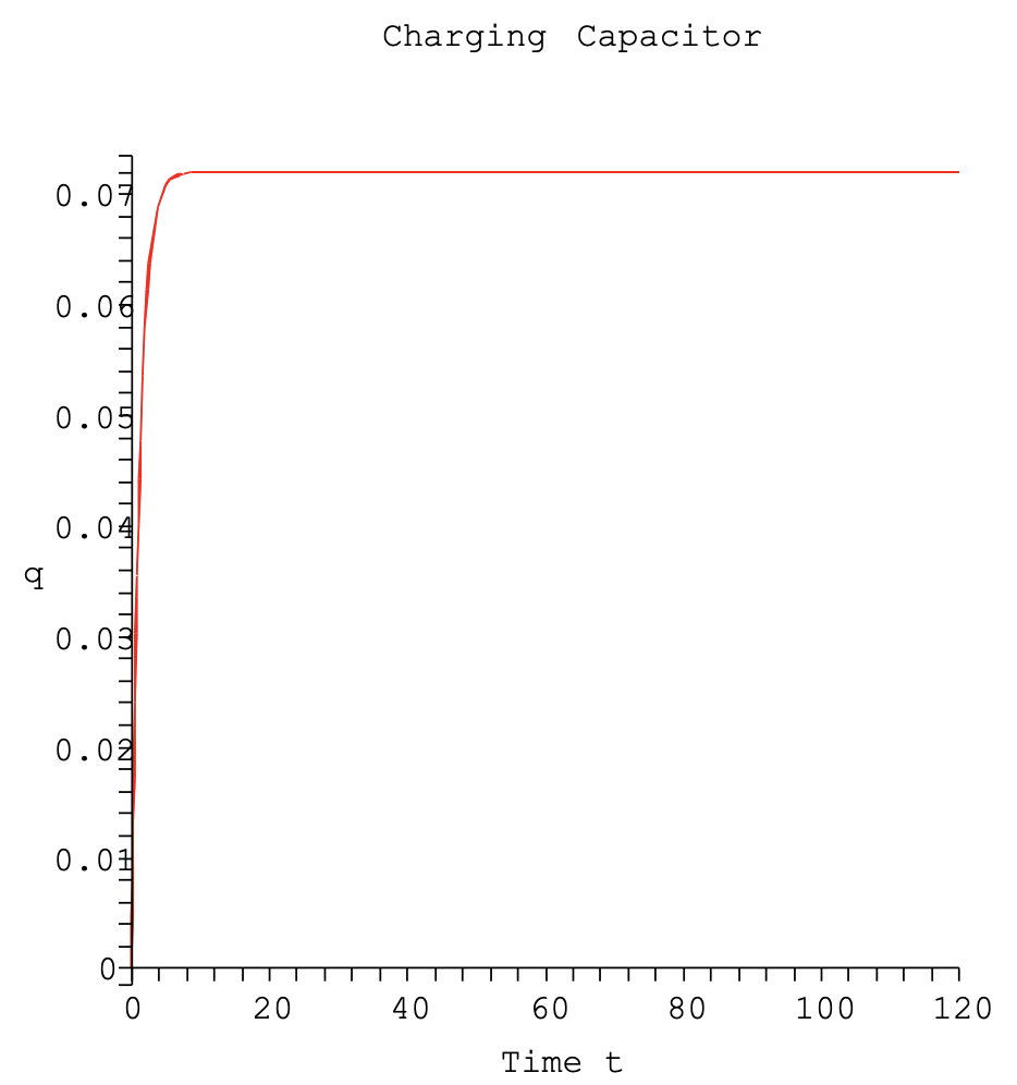
Now we can study the behavior of this solution. For large times the second term goes to zero. Thus, the capacitor charges up, asymptotically, to the final value of \(q_0 = CV_0\). This is what we expect, because the current is no longer flowing over \(R\) and this just gives the relation between the potential difference across the capacitor plates when a charge of \(q_0\) is established on the plates.

Figure 2.21. The charge as a function of time for a charging capacitor with \(R=2.00\) \(\mathrm{k} \Omega, C=6.00 \mathrm{mF}\), and \(V_{0}=12 \mathrm{~V}\).

Let's put in some values for the parameters. We let \(R=2.00 \mathrm{k} \Omega, C=6.00\) \(\mathrm{mF}\), and \(V_{0}=12 \mathrm{~V}\). A plot of the solution is given in Figure 2.21. We see that the charge builds up to the value of \(C V_{0}=72 \mathrm{mC}\). If we use a smaller resistance, \(R=200 \Omega\), we see in Figure 2.22 that the capacitor charges to the same value, but much faster.

The rate at which a capacitor charges, or discharges, is governed by the time constant, \(\tau=R C\). This is the constant factor in the exponential. The larger it is, the slower the exponential term decays. If we set \(t=\tau\), we find that

\[q(\tau)=C V_{0}\left(1-e^{-1}\right)=(1-0.3678794412 \ldots) q_{0} \approx 0.63 q_{0} \nonumber \]

Thus, at time \(t = \tau\), the capacitor has almost charged to two thirds of its final value. For the first set of parameters, \(\tau = 12s\). For the second set, \(\tau = 1.2s\).

Figure 2.22. The charge as a function of time for a charging capacitor with \(R=200\) \(\Omega, C=6.00 \mathrm{mF}\), and \(V_{0}=12 \mathrm{~V}\).

Now, let's assume the capacitor is charged with charge \(\pm q_{0}\) on its plates. If we disconnect the battery and reconnect the wires to complete the circuit, the charge will then move off the plates, discharging the capacitor. The relevant form of our initial value problem becomes

\[R \dfrac{d q}{d t}+\dfrac{q}{C}=0, \quad q(0)=q_{0} \label{2.93} \]

This equation is simpler to solve. Rearranging, we have

\[\dfrac{d q}{d t}=-\dfrac{q}{R C} \label{2.94} \]

This is a simple exponential decay problem, which you can solve using separation of variables. However, by now you should know how to immediately write down the solution to such problems of the form \(y^{\prime}=k y\). The solution is

\[q(t)=q_{0} e^{-t / \tau}, \quad \tau=R C \nonumber \]

We see that the charge decays exponentially. In principle, the capacitor never fully discharges. That is why you are often instructed to place a shunt across a discharged capacitor to fully discharge it.

In Figure 2.23 we show the discharging of our two previous RC circuits.

Once again, \(\tau = RC\) determines the behavior. At \(t = \tau\) we have

\[q(\tau) = q_0e^{-1} = (0.3678794412...)q_0 \approx 0.37q_0. \nonumber \]

So, at this time the capacitor only has about a third of its original value.

Figure 2.23. The charge as a function of time for a discharging capacitor with \(R = 2.00\) \(k \Omega\) or \(R = 200 \Omega\), and \(C = 6.00 mF\), and \(q_0 = 72 mC\).

Example 2.20. LC Circuits

Another simple result comes from studying LC circuits. We will now connect a charged capacitor to an inductor. In this case, we consider the initial value problem

\[L \ddot{q}+\dfrac{1}{C} q=0, \quad q(0)=q_{0}, \dot{q}(0)=I(0)=0 \label{2.95} \]

Dividing out the inductance, we have

\[\ddot{q}+\dfrac{1}{L C} q=0 \label{2.96} \]

This equation is a second order, constant coefficient equation. It is of the same form as the one we saw earlier for simple harmonic motion of a mass on a spring. So, we expect oscillatory behavior. The characteristic equation is

\[r^{2}+\dfrac{1}{L C}=0 \nonumber \]

The solutions are

\[r_{1,2}=\pm \dfrac{i}{\sqrt{L C}} \nonumber \]

Thus, the solution of (2.96) is of the form

\[q(t)=c_{1} \cos (\omega t)+c_{2} \sin (\omega t), \quad \omega=(L C)^{-1 / 2} \label{2.97} \]

Inserting the initial conditions yields

\[q(t)=q_{0} \cos (\omega t) \label{2.98} \]

The oscillations that result are understandable. As the charge leaves the plates, the changing current induces a changing magnetic field in the inductor. The stored electrical energy in the capacitor changes to stored magnetic energy in the inductor. However, the process continues until the plates are charged with opposite polarity and then the process begins in reverse. The charged capacitor then discharges and the capacitor eventually returns to its original state and the whole system repeats this over and over.

The frequency of this simple harmonic motion is easily found. It is given by

\[f=\dfrac{\omega}{2 \pi}=\dfrac{1}{2 \pi} \dfrac{1}{\sqrt{L C}} \label{2.99} \]

This is called the tuning frequency because of its role in tuning circuits.

Of course, this is an ideal situation. There is always resistance in the circuit, even if only a small amount from the wires. So, we really need to account for resistance, or even add a resistor. This leads to a slightly more complicated system in which damping will be present.

More complicated circuits are possible by looking at parallel connections, or other combinations, of resistors, capacitors and inductors. This will result in several equations for each loop in the circuit, leading to larger systems of differential equations. an example of another circuit setup is shown in Figure 2.24. This is not a problem that can be covered in the first year physics course.

Figure 2.24. A circuit with two loops containing several different circuit elements.

There are two loops, indicated in Figure 2.25 as traversed clockwise. For each loop we need to apply Kirchoff's Loop Rule. There are three oriented currents, labeled \(I_{i}, i=1,2,3\). Corresponding to each current is a changing charge, \(q_{i}\) such that

\[I_{i}=\dfrac{d q_{i}}{d t}, \quad i=1,2,3 \nonumber \]

For loop one we have

\[I_{1} R_{1}+\dfrac{q_{2}}{C}=V(t) \label{2.100} \]

For loop two

\[I_{3} R_{2}+L \dfrac{d I_{3}}{d t}=\dfrac{q_{2}}{C} \label{2.101} \]

Figure 2.25. The previous parallel circuit with the directions indicated for traversing the loops in Kirchoff's Laws.

We have three unknown functions for the charge. Once we know the charge functions, differentiation will yield the currents. However, we only have two equations. We need a third equation. This is found from Kirchoff’s Point (Junction) Rule. Consider the points A and B in Figure 2.25. Any charge (current) entering these junctions must be the same as the total charge (current) leaving the junctions. For point A we have

\[I_{1}=I_{2}+I_{3} \label{2.102} \]

or

\[\dot{q}_{1}=\dot{q}_{2}+\dot{q}_{3} \label{2.103} \]

Equations (2.100), (2.101), and (2.103) form a coupled system of differential equations for this problem. There are both first and second order derivatives involved. We can write the whole system in terms of charges as

\[\begin{array}{r}
R_{1} \dot{q}_{1}+\dfrac{q_{2}}{C}=V(t) \\
R_{2} \dot{q}_{3}+L \ddot{q}_{3}=\dfrac{q_{2}}{C} \\
\dot{q}_{1}=\dot{q}_{2}+\dot{q}_{3}
\end{array} \label{2.104} \]

The question is whether, or not, we can write this as a system of first order differential equations. Since there is only one second order derivative, we can introduce the new variable \(q_{4}=\dot{q}_{3}\). The first equation can be solved for \(\dot{q}_{1}\). The third equation can be solved for \(\dot{q}_{2}\) with appropriate substitutions for the other terms. \(\dot{q}_{3}\) is gotten from the definition of \(q_{4}\) and the second equation can be solved for \(\ddot{q}_{3}\) and substitutions made to obtain the system

\begin{aligned}
\dot{q}_{1} &=\dfrac{V}{R_{1}}-\dfrac{q_{2}}{R_{1} C} \\
\dot{q}_{2} &=\dfrac{V}{R_{1}}-\dfrac{q_{2}}{R_{1} C}-q_{4} \\
\dot{q}_{3} &=q_{4} \\
\dot{q}_{4} &=\dfrac{q_{2}}{L C}-\dfrac{R_{2}}{L} q_{4}
\end{aligned}

So, we have a nonhomogeneous first order system of differential equations. In the last section we learned how to solve such systems.

2.9.3 Love Affairs

The next application is one that has been studied by several authors as a cute system involving relationships. One considers what happens to the affections that two people have for each other over time. Let \(R\) denote the affection that Romeo has for Juliet and \(J\) be the affection that Juliet has for Romeo. positive values indicate love and negative values indicate dislike.

One possible model is given by

\[\begin{aligned}
\dfrac{d R}{d t} &=b J \\
\dfrac{d J}{d t} &=c R
\end{aligned} \label{2.105} \]

with \(b>0\) and \(c<0\). In this case Romeo loves Juliet the more she likes him. But Juliet backs away when she finds his love for her increasing.

A typical system relating the combined changes in affection can be modeled as

\[\begin{aligned}
&\dfrac{d R}{d t}=a R+b J \\
&\dfrac{d J}{d t}=c R+d J
\end{aligned} \label{2.106} \]

Several scenarios are possible for various choices of the constants. For example, if \(a>0\) and \(b>0\), Romeo gets more and more excited by Juliet's love for him. If \(c>0\) and \(d<0\), Juliet is being cautious about her relationship with Romeo. For specific values of the parameters and initial conditions, one can explore this match of an overly zealous lover with a cautious lover.

2.9.4 Predator Prey Models

Another common model studied is that of competing species. For example, we could consider a population of rabbits and foxes. Left to themselves, rabbits would tend to multiply, thus

\(\dfrac{d R}{d t}=a R\),

with \(a>0\). In such a model the rabbit population would grow exponentially. Similarly, a population of foxes would decay without the rabbits to feed on. So, we have that

\[\dfrac{d F}{d t}=-b F \nonumber \]

for \(b>0\).
Now, if we put these populations together on a deserted island, they would interact. The more foxes, the rabbit population would decrease. However, the more rabbits, the foxes would have plenty to eat and the population would thrive. Thus, we could model the competing populations as

\[\begin{gathered}
\dfrac{d R}{d t}=a R-c F \\
\dfrac{d F}{d t}=-b F+d R
\end{gathered} \label{2.107} \]

where all of the constants are positive numbers. Studying this coupled system would lead to as study of the dynamics of these populations. We will discuss other (nonlinear) systems in the next chapter.

2.9.5 Mixture Problems

There are many types of mixture problems. Such problems are standard in a first course on differential equations as examples of first order differential equations. Typically these examples consist of a tank of brine, water containing a specific amount of salt with pure water entering and the mixture leaving, or the flow of a pollutant into, or out of, a lake.

In general one has a rate of flow of some concentration of mixture entering a region and a mixture leaving the region. The goal is to determine how much stuff is in the region at a given time. This is governed by the equation

Rate of change of substance = Rate In − Rate Out.

This can be generalized to the case of two interconnected tanks. We provide some examples.

Example 2.21. Single Tank Problem

A 50 gallon tank of pure water has a brine mixture with concentration of 2 pounds per gallon entering at the rate of 5 gallons per minute. [See Figure 2.26.] At the same time the well-mixed contents drain out at the rate of 5 gallons per minute. Find the amount of salt in the tank at time t. In all such problems one assumes that the solution is well mixed at each instant of time.

Figure 2.26. A typical mixing problem.

Let \(x(t)\) be the amount of salt at time \(t\). Then the rate at which the salt in the tank increases is due to the amount of salt entering the tank less that leaving the tank. To figure out these rates, one notes that \(dx/dt\) has units of pounds per minute. The amount of salt entering per minute is given by the product of the entering concentration times the rate at which the brine enters. This gives the correct units:

\[\left(2 \dfrac{\text { pounds }}{\text { gal }}\right)\left(5 \dfrac{\text { gal }}{\min }\right)=10 \dfrac{\text { pounds }}{\min }. \nonumber \]

Similarly, one can determine the rate out as

\[\left(\dfrac{x \text { pounds }}{50 \text { gal }}\right)\left(5 \dfrac{\text { gal }}{\min }\right)=\dfrac{x}{10} \dfrac{\text { pounds }}{\min } \nonumber \]

Thus, we have

\[\dfrac{d x}{d t}=10-\dfrac{x}{10} \nonumber \]

This equation is easily solved using the methods for first order equations.

Example 2.22. Double Tank Problem

Figure 2.27. The two tank problem.

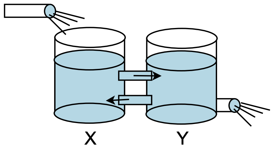
One has two tanks connected together, labelled tank \(X\) and tank \(Y\), as shown in Figure 2.27. Let tank \(X\) initially have 100 gallons of brine made with 100 pounds of salt. Tank \(Y\) initially has 100 gallons of pure water. Now pure water is pumped into tank \(X\) at a rate of 2.0 gallons per minute. Some of the mixture of brine and pure water flows into tank \(Y\) at 3 gallons per minute. To keep the tank levels the same, one gallon of the \(Y\) mixture flows back into tank \(X\) at a rate of one gallon per minute and 2.0 gallons per minute drains out. Find the amount of salt at any given time in the tanks. What happens over a long period of time?

In this problem we set up two equations. Let \(x(t)\) be the amount of salt in tank \(X\) and \(y(t)\) the amount of salt in tank \(Y\). Again, we carefully look at the rates into and out of each tank in order to set up the system of differential equations. We obtain the system

\[\begin{aligned}
\dfrac{d x}{d t} &=\dfrac{y}{100}-\dfrac{3 x}{100} \\
\dfrac{d y}{d t} &=\dfrac{3 x}{100}-\dfrac{3 y}{100}
\end{aligned} \label{2.108} \]

This is a linear, homogenous constant coefficient system of two first order equations, which we know how to solve.

2.9.6 Chemical Kinetics

There are many problems that come from studying chemical reactions. The simplest reaction is when a chemical \(A\) turns into chemical \(B\). This happens at a certain rate, \(k>0\). This can be represented by the chemical formula

\[A \underset{k}{\longrightarrow} B \nonumber \]

In this case we have that the rates of change of the concentrations of \(A,[A]\), and \(B,[B]\), are given by

\[\begin{aligned}
\dfrac{d[A]}{d t} &=-k[A] \\
\dfrac{d[B]}{d t} &=k[A]
\end{aligned} \label{2.109} \]

Think about this as it is a key to understanding the next reactions.
A more complicated reaction is given by

\[A \underset{k_{1}}{\longrightarrow} B \underset{k_{2}}{\longrightarrow} C \nonumber \]

In this case we can add to the above equation the rates of change of concentrations \([B]\) and \([C]\). The resulting system of equations is

\[\begin{aligned}
\dfrac{d[A]}{d t} &=-k_{1}[A] \\
\dfrac{d[B]}{d t} &=k_{1}[A]-k_{2}[B], \\
\dfrac{d[C]}{d t} &=k_{2}[B]
\end{aligned} \label{2.110} \]

One can further consider reactions in which a reverse reaction is possible. Thus, a further generalization occurs for the reaction

\[A \underset{k_{1}}{\stackrel{k_{3}}{\longrightarrow}} B \underset{k_{2}}{\longrightarrow} C \nonumber \]

The resulting system of equations is

\[\begin{aligned}
\dfrac{d[A]}{d t} &=-k_{1}[A]+k_{3}[B], \\
\dfrac{d[B]}{d t} &=k_{1}[A]-k_{2}[B]-k_{3}[B], \\
\dfrac{d[C]}{d t} &=k_{2}[B] .
\end{aligned} \label{2.111} \]

More complicated chemical reactions will be discussed at a later time.

2.9.7 Epidemics

Another interesting area of application of differential equation is in predicting the spread of disease. Typically, one has a population of susceptible people or animals. Several infected individuals are introduced into the population and one is interested in how the infection spreads and if the number of infected people drastically increases or dies off. Such models are typically nonlinear and we will look at what is called the SIR model in the next chapter. In this section we will model a simple linear model.

Let break the population into three classes. First, \(S(t)\) are the healthy people, who are susceptible to infection. Let \(I(t)\) be the number of infected people. Of these infected people, some will die from the infection and others recover. Let’s assume that initially there in one infected person and the rest, say \(N\), are obviously healthy. Can we predict how many deaths have occurred by time \(t\)?

Let’s try and model this problem using the compartmental analysis we had seen in the mixing problems. The total rate of change of any population would be due to those entering the group less those leaving the group. For example, the number of healthy people decreases due infection and can increase when some of the infected group recovers. Let’s assume that the rate of infection is proportional to the number of healthy people,\(aS\). Also, we assume that the number who recover is proportional to the number of infected, \(rI\). Thus, the rate of change of the healthy people is found as

\[\dfrac{d S}{d t}=-a S+r I. \nonumber \]

Let the number of deaths be \(D(t)\). Then, the death rate could be taken to be proportional to the number of infected people. So,

\[\dfrac{d D}{d t}=d I \nonumber \]

Finally, the rate of change of infectives is due to healthy people getting infected and the infectives who either recover or die. Using the corresponding terms in the other equations, we can write

\[\dfrac{d I}{d t}=a S-r I-d I \nonumber \]

This linear system can be written in matrix form.

\[\dfrac{d}{d t}\left(\begin{array}{c}
S \\
I \\
D
\end{array}\right)=\left(\begin{array}{ccc}
-a & r & 0 \\
a & -d-r & 0 \\
0 & d & 0
\end{array}\right)\left(\begin{array}{l}
S \\
I \\
D
\end{array}\right) \label{2.112} \]

The eigenvalue equation for this system is

\[\lambda\left[\lambda^{2}+(a+r+d) \lambda+a d\right]=0. \nonumber \]

The reader can find the solutions of this system and determine if this is a realistic model.