3.2: Autonomous First Order Equations

In this section we will review the techniques for studying the stability of nonlinear first order autonomous equations. We will then extend this study to looking at families of first order equations which are connected through a parameter

Recall that a first order autonomous equation is given in the form

\[\dfrac{dy}{dt} = f(y). \nonumber \]

We will assume that \(f\) and \(\dfrac{\partial f}{\partial y}\) are continuous functions of \(y\), so that we know that solutions of initial value problems exist and are unique.

We will recall the qualitative methods for studying autonomous equations by considering the example

\[\dfrac{d y}{d t}=y-y^{2} \label{3.3} \]

This is just an example of a logistic equation.

First, one determines the equilibrium, or constant, solutions given by \(y^{\prime}= 0\). For this case, we have \(y-y^{2}=0\). So, the equilibrium solutions are \(y=0\) and \(y=1\). Sketching these solutions, we divide the \(t y\)-plane into three regions. Solutions that originate in one of these regions at \(t=t_{0}\) will remain in that region for all \(t>t_{0}\) since solutions cannot intersect. [Note that if two solutions intersect then they have common values \(y_{1}\) at time \(t_{1}\). Using this information, we could set up an initial value problem for which the initial condition is \(y\left(t_{1}\right)=y_{1}\). Since the two different solutions intersect at this point in the phase plane, we would have an initial value problem with two different solutions corresponding to the same initial condition. This contradicts the uniqueness assumption stated above. We will leave the reader to explore this further in the homework.]

Next, we determine the behavior of solutions in the three regions. Noting that \(d y / d t\) gives the slope of any solution in the plane, then we find that the solutions are monotonic in each region. Namely, in regions where \(d y / d t>0\), we have monotonically increasing functions. We determine this from the right side of our equation.

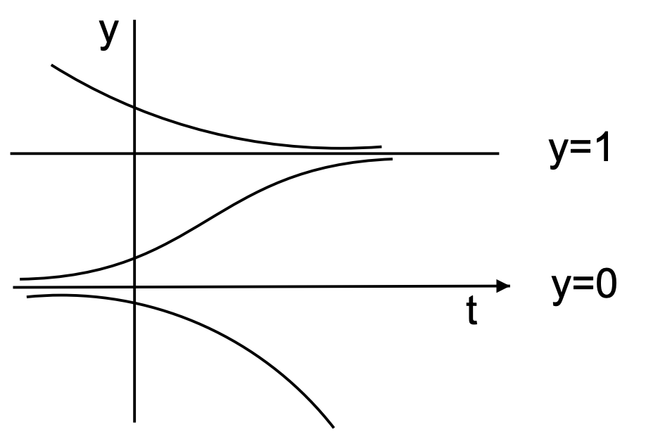
For example, in this problem \(y-y^{2}>0\) only for the middle region and \(y-y^{2}<0\) for the other two regions. Thus, the slope is positive in the middle region, giving a rising solution as shown in Figure 3.1. Note that this solution does not cross the equilibrium solutions. Similar statements can be made about the solutions in the other regions.

We further note that the solutions on either side of \(y = 1\) tend to approach this equilibrium solution for large values of \(t\). In fact, no matter how close one is to \(y = 1\), eventually one will approach this solution as \(t → ∞\). So, the equilibrium solution is a stable solution. Similarly, we see that \(y = 0\) is an unstable equilibrium solution.

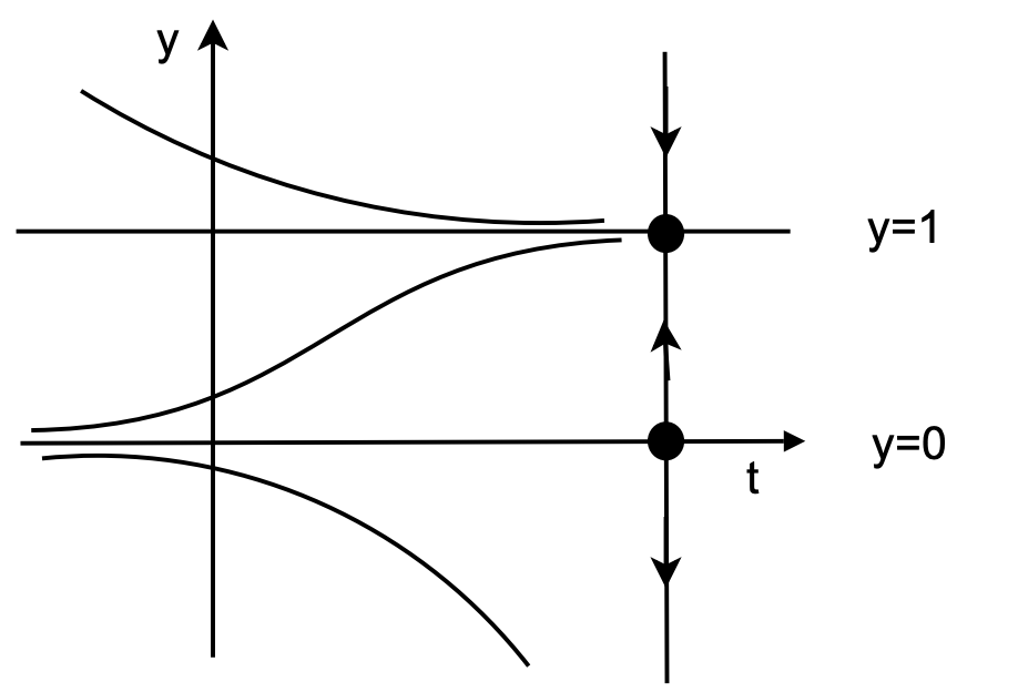
If we are only interested in the behavior of the equilibrium solutions, we could just construct a phase line. In Figure 3.2 we place a vertical line to the right of the \(ty\)-plane plot. On this line one first places dots at the corresponding equilibrium solutions and labels the solutions. These points at the equilibrium solutions are end points for three intervals. In each interval one then places arrows pointing upward (downward) indicating solutions with positive (negative) slopes. Looking at the phase line one can now determine if a given equilibrium is stable (arrows pointing towards the point) or unstable

Figure 3.1. Representative solution behavior for \(y' = y - y^2\).

(arrows pointing away from the point). In Figure 3.3 we draw the final phase line by itself.

Figure 3.2. Representative solution behavior and phase line for \(y' = y - y^2\).