3.4: Bifurcations for First Order Equations

In this section we introduce families of first order differential equations of the form

\[\dfrac{d y}{d t}=f(y ; \mu) \nonumber \]

Here \(\mu\) is a parameter that we can change and then observe the resulting effects on the behaviors of the solutions of the differential equation. When a small change in the parameter leads to large changes in the behavior of the solution, then the system is said to undergo a bifurcation. We will turn to some generic examples, leading to special bifurcations of first order autonomous differential equations.

Example 3.1. \(y' = y^2 - \mu\).

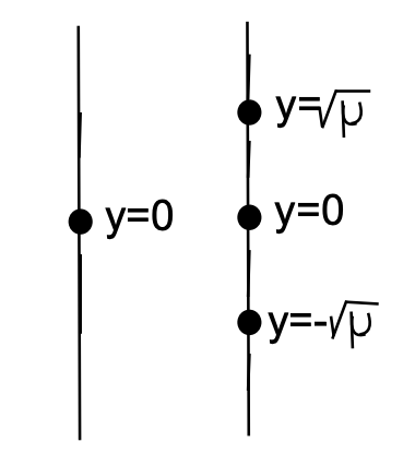
First note that equilibrium solutions occur for \(y^{2}=\mu\). In this problem, there are three cases to consider.

1. \(\mu>0\).
   In this case there are two real solutions, \(y=\pm \sqrt{\mu}\). Note that \(y^{2}-\mu<0\) for \(|y|<\sqrt{\mu}\). So, we have the left phase line in Figure 3.4.
2. \(\mu=0\).
   There is only one equilibrium point at \(y=0\). The equation becomes \(y^{\prime}=y^{2}\). It is obvious that the right side of this equation is never negative.
   So, the phase line is shown as the middle line in Figure 3.4.
3. \(\mu<0\).
   In this case there are no equilibrium solutions. Since \(y^{2}-\mu>0\), the slopes for all solutions are positive as indicated by the last phase line in Figure 3.4.

Figure 3.4. Phase lines for \(y^{\prime}=y^{2}-\mu\). On the left \(\mu>0\) and on the right \(\mu<0\).

We can combine these results into one diagram known as a bifurcation diagram. We plot the equilibrium solutions \(y\) vs \(\mu\). We begin by lining up the phase lines for various \(\mu\)'s. We display these in Figure 3.5. Note the pattern of equilibrium points satisfies \(y=\mu^{2}\) as it should. This is easily seen to be a parabolic curve. The upper branch of this curve is a collection of unstable equilibria and the bottom is a stable branch. So, we can dispose of the phase lines and just keep the equilibria. However, we will draw the unstable branch as a dashed line and the stable branch as a solid line.

The bifurcation diagram is displayed in Figure 3.6. This type of bifurcation is called a saddle-node bifurcation. The point \(\mu=0\) at which the behavior changes is called the bifurcation point. As \(\mu\) goes from negative to positive, we go from having no equilibria to having one stable and one unstable equilibrium point.

Example 3.2. \(y' = y^2 - \mu y\).

In this example we have two equilibrium points, \(y=0\) and \(y=\mu\). The behavior of the solutions depends upon the sign of \(y^{2}-\mu y=y(y-\mu)\). This leads to four cases with the indicated signs of the derivative.

1. \(y>0, y-\mu>0 \Rightarrow y^{\prime}>0\).
2. \(y<0, y-\mu>0 \Rightarrow y^{\prime}<0\).
3. \(y>0, y-\mu<0 \Rightarrow y^{\prime}<0\).
4. \(y<0, y-\mu<0 \Rightarrow y^{\prime}>0\).

The corresponding phase lines and superimposed bifurcation diagram are shown in 3.7. The bifurcation diagram is in Figure 3.8 and this is called a transcritical bifurcation.

Figure 3.5. The typical phase lines for \(y' = y^2 - \mu\).

Figure 3.6. Bifurcation diagram for \(y' = y^2 - \mu\). This is an example of a saddle-node bifurcation.

Figure 3.7. Collection of phase lines for \(y' = y^2 - \mu y\).

Example 3.3. \(y' = y^3 - \mu y\).

For this last example, we find from \(y^3 - \mu y = y(y^2 - \mu) = 0\) that there are two cases.

1. \(\mu < 0\) In this case there is only one equilibrium point at \(y = 0\). For positive values of \(y\) we have that \(y' > 0\) and for negative values of \(y\) we have that \(y'<0\). Therefore, this is an unstable equilibrium point.

Figure 3.8. Bifurcation diagram for \(y' = y^2 - \mu y\). This is an example of a transcritical bifurcation.

2. \(\mu>0\) Here we have three equilibria, \(x=0, \pm \sqrt{\mu}\). A careful investigation shows that \(x=0\). is a stable equilibrium point and that the other two equilibria are unstable.

In Figure 3.9 we show the phase lines for these two cases. The corresponding bifurcation diagram is then sketched in Figure 3.10. For obvious reasons this has been labeled a pitchfork bifurcation.

Figure 3.9. The phase lines for \(y' = y^3 - \mu y\). The left one corresponds to \(\mu < 0\) and the right phase line is for \(\mu > 0\)

Figure 3.10. Bifurcation diagram for \(y' = y^3 - \mu y\). This is an example of a pitchfork burification.