10.3: Gamma Function

For \(\nu\) not an integer the recursion relation for the Bessel function generates something very similar to factorials. These quantities are most easily expressed in something called a Gamma-function, defined as

\[\Gamma(\nu) = \int_0^\infty e^{-t}t^{\nu-1} dt,\;\;\;\nu>0.\]

Some special properties of \(\Gamma\) function now follow immediately:

\[\begin{aligned} \Gamma(1) & = & \int_0^\infty e^{-t}dt = \left.-e^{-1}\right|^\infty_0 =1-e^{-\infty}=1\nonumber\\ \Gamma(\nu) & = & \int_0^\infty e^{-t} t^{\nu-1} dt = -\int_0^\infty \frac{de^{-t}}{dt} t^{\nu-1} dt\nonumber\\ &=& \left.- e^{-t} t^{\nu-1} \right|^\infty_0 +(\nu-1) \int_0^\infty e^{-t} t^{\nu-2} dt \end{aligned}\]

The first term is zero, and we obtain \[\Gamma(\nu) = (\nu-1)\Gamma(\nu-1)\]

From this we conclude that

\[\Gamma(2)=1\cdot1=1,\;\Gamma(3)=2\cdot1\cdot1=2,\; \Gamma(4)=3\cdot2\cdot1\cdot1=2,\;\Gamma(n) = (n-1)!.\]

Thus for integer argument the \(\Gamma\) function is nothing but a factorial, but it also defined for other arguments. This is the sense in which \(\Gamma\) generalises the factorial to non-integer arguments. One should realize that once one knows the \(\Gamma\) function between the values of its argument of, say, 1 and 2, one can evaluate any value of the \(\Gamma\) function through recursion. Given that \(\Gamma(1.65) = 0.9001168163\) we find

\[\Gamma(3.65) = 2.65\times1.65\times0.9001168163 = 3.935760779 .\]

Exercise \(\PageIndex{1}\)

Evaluate \(\Gamma(3)\), \(\Gamma(11)\), \(\Gamma(2.65)\).

Answer

\(2!=2\), \(10!=3628800\), \(1.65\times0.9001168163=1.485192746\).

We also would like to determine the \(\Gamma\) function for \(\nu<1\). One can invert the recursion relation to read \[\Gamma(\nu-1) = \frac{\Gamma(\nu)}{\nu-1},\] \(\Gamma(0.7) = \Gamma(1.7)/0.7=0.909/0.7=1.30\).

What is \(\Gamma(\nu)\) for \(\nu<0\)? Let us repeat the recursion derived above and find \[\Gamma(-1.3) = \frac{\Gamma(-0.3)}{-1.3} = \frac{\Gamma(0.7)}{-1.3\times -0.3} = \frac{\Gamma(1.7)}{0.7\times-0.3\times -1.3}=3.33\;.\] This works for any value of the argument that is not an integer. If the argument is integer we get into problems. Look at \(\Gamma(0)\). For small positive \(\epsilon\) \[\Gamma(\pm\epsilon)= \frac{\Gamma(1\pm\epsilon)}{\pm\epsilon} =\pm \frac{1}{\epsilon}\rightarrow \pm \infty.\] Thus \(\Gamma(n)\) is not defined for \(n\leq0\). This can be easily seen in the graph of the \(\Gamma\) function, Fig. \(\PageIndex{1}\).

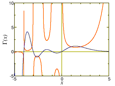
Figure \(\PageIndex{1}\): A graph of the \(\Gamma\) function (solid line). The inverse \(1/\Gamma\) is also included (dashed line). Note that this last function is not discontinuous.

Finally, in physical problems one often uses \(\Gamma(1/2)\), \[\Gamma(\frac{1}{2}) = \int_0^\infty e^{-t}t^{-1/2} dt = 2\int_0^\infty e^{-t}dt^{1/2} = 2\int_0^\infty e^{-x^2}dx.\] This can be evaluated by a very smart trick, we first evaluate \(\Gamma(1/2)^2\) using polar coordinates \[\begin{aligned} \Gamma(\frac{1}{2})^2 &=& 4 \int_0^\infty e^{-x^2}dx\int_0^\infty e^{-y^2}dy \nonumber\\ &=& 4 \int_0^\infty \int_0^{\pi/2} e^{-\rho^2}\rho d\rho d\phi = \pi.\end{aligned}\] (See the discussion of polar coordinates in Sec. 7.1.) We thus find \[\Gamma(1/2)=\sqrt{\pi},\;\;\Gamma(3/2)=\frac{1}{2}\sqrt{\pi},\;\;{\rm etc.}\]