12.2: The Wave Equation
- Page ID
- 9468
In this section we consider initial-boundary value problems of the form
\[\label{eq:12.2.1} \begin{array}{c}{u_{tt}=a^{2}u_{xx},\quad 0<x<L,\quad t>0,}\\{u(0,t)=0,\quad u(L,t)=0,\quad t>0,}\\{u(x,0)=f(x),\quad u_{t}(x,0)=g(x),\quad 0\leq x\leq L,}\end{array}\]
where \(a\) is a constant and \(f\) and \(g\) are given functions of \(x\). The partial differential equation \(u_{tt}=a^2u_{xx}\) is called the wave equation. It is necessary to specify both \(f\) and \(g\) because the wave equation is a second order equation in \(t\) for each fixed \(x\). This equation and its generalizations
\[u_{tt}=a^2(u_{xx}+u_{yy}) \quad \text{and} \quad u_{tt}=a^2(u_{xx}+u_{yy}+u_{zz}) \nonumber \]
to two and three space dimensions have important applications to the the propagation of electromagnetic, sonic, and water waves.
The Vibrating String
We motivate the study of the wave equation by considering its application to the vibrations of a string – such as a violin string – tightly stretched in equilibrium along the \(x\)-axis in the \(xu\)-plane and tied to the points \((0,0)\) and \((L,0)\) (Figure 12.2.1 ).

If the string is plucked in the vertical direction and released at time \(t=0\), it will oscillate in the \(xu\)-plane. Let \(u(x,t)\) denote the displacement of the point on the string above (or below) the abscissa \(x\) at time \(t\).
We’ll show that it is reasonable to assume that \(u\) satisfies the wave equation under the following assumptions:
- The mass density (mass per unit length) \(\rho\) of the string is constant throughout the string.
- The tension \(T\) induced by tightly stretching the string along the \(x\)-axis is so great that all other forces, such as gravity and air resistance, can be neglected.
- The tension at any point on the string acts along the tangent to the string at that point, and the magnitude of its horizontal component is always equal to \(T\), the tension in the string in equilibrium.
- The slope of the string at every point remains sufficiently small so that we can make the approximation \[\label{eq:12.2.2} \sqrt{1+u_x^2}\approx1.\]
Figure 12.2.2 shows a segment of the displaced string at a time \(t>0\). (Don’t think that the figure is necessarily inconsistent with Assumption 4; we exaggerated the slope for clarity.)
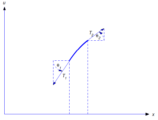
The vectors \({\bf T}_1\) and \({\bf T}_2\) are the forces due to tension, acting along the tangents to the segment at its endpoints. From Newton’s second law of motion, \({\bf T}_1-{\bf T}_2\) is equal to the mass times the acceleration of the center of mass of the segment. The horizontal and vertical components of \({\bf T}_1-{\bf T}_2\) are
\[|{\bf T}_2|\cos\theta_2- |{\bf T}_1|\cos\theta_1 \quad \text{and} \quad |{\bf T}_2|\sin\theta_2- |{\bf T}_1|\sin\theta_1, \nonumber \]
respectively. Since
\[\label{eq:12.2.3} |{\bf T}_2|\cos\theta_2=|{\bf T}_1|\cos\theta_1=T\]
by assumption, the net horizontal force is zero, so there’s no horizontal acceleration. Since the initial horizontal velocity is zero, there’s no horizontal motion.
Applying Newton’s second law of motion in the vertical direction yields
\[\label{eq:12.2.4} |{\bf T}_2|\sin\theta_2- |{\bf T}_1|\sin\theta_1=\rho\Delta s\,u_{tt}(\overline x,t),\]
where \(\Delta s\) is the length of the segment and \(\overline x\) is the abscissa of the center of mass; hence,
\[x<\overline x <x+\Delta x.\nonumber\]
From calculus, we know that
\[\Delta s=\int_x^{x+\Delta x}\sqrt{1+u_x^2(\sigma,t)}\,d\sigma;\nonumber\]
however, because of Equation \ref{eq:12.2.2}, we make the approximation
\[\Delta s\approx\int_x^{x+\Delta x}1\,d\sigma=\Delta x,\nonumber\]
so Equation \ref{eq:12.2.4} becomes
\[|{\bf T}_2|\sin\theta_2- |{\bf T}_1|\sin\theta_1=\rho\Delta x\,u_{tt}(\overline x,t).\nonumber\]
Therefore
\[{|{\bf T}_2|\sin\theta_2- |{\bf T}_1|\sin\theta_1\over\Delta x}=\rho u_{tt}(\overline x,t).\nonumber\]
Recalling Equation \ref{eq:12.2.3}, we divide by \(T\) to obtain
\[\label{eq:12.2.5} {\tan\theta_2-\tan\theta_1\over\Delta x}= {\rho\over T}u_{tt}(\overline x,t).\]
Since \(\tan\theta_1=u_x(x,t)\) and \(\tan\theta_2=u_x(x+\Delta x,t)\), Equation \ref{eq:12.2.5} is equivalent to
\[{u_x(x+\Delta x)-u_x(x,t)\over \Delta x}= {\rho\over T}u_{tt}(\overline x,t).\nonumber\]
Letting \(\Delta x\to 0\) yields
\[u_{xx}(x,t)={\rho\over T}u_{tt}(x,t),\nonumber\]
which we rewrite as \(u_{tt}=a^2u_{xx}\), with \(a^2=T/\rho\).
The Formal Solution
As in Section 12.1, we use separation of variables to obtain a suitable definition for the formal solution of Equation \ref{eq:12.2.1}. We begin by looking for functions of the form \(v(x,t)=X(x)T(t)\) that are not identically zero and satisfy
\[v_{tt}=a^2v_{xx},\quad v(0,t)=0,\quad v(L,t)=0\nonumber\]
for all \((x,t)\). Since
\[v_{tt}=XT''\quad \text{and} \quad v_{xx}=X''T,\nonumber\]
\(v_{tt}=a^2v_{xx}\) if and only if
\[XT''=a^2X''T,\nonumber\]
which we rewrite as
\[{T''\over a^2T}={X''\over X}.\nonumber\]
For this to hold for all \((x,t)\), the two sides must equal the same constant; thus,
\[{X''\over X}={T''\over a^2T}=-\lambda,\nonumber\]
which is equivalent to
\[X''+\lambda X=0\nonumber\]
and
\[\label{eq:12.2.6} T''+a^2\lambda T=0.\]
Since \(v(0,t)=X(0)T(t)=0\) and \(v(L,t)=X(L)T(t)=0\) and we don’t want \(T\) to be identically zero, \(X(0)=0\) and \(X(L)=0\). Therefore \(\lambda\) must be an eigenvalue of
\[\label{eq:12.2.7} X''+\lambda X=0,\quad X(0)=0,\quad X(L)=0,\]
and \(X\) must be a \(\lambda\)-eigenfunction. From Theorem 11.1.2, the eigenvalues of Equation \ref{eq:12.2.7} are \(\lambda_n=n^2\pi^2/L^2\), with associated eigenfunctions
\[X_n=\sin{n\pi x\over L}, \quad n=1,2,3,\dots.\nonumber\]
Substituting \(\lambda=n^2\pi^2/L^2\) into Equation \ref{eq:12.2.6} yields
\[T''+(n^2\pi^2a^2/L^2)T=0,\nonumber\]
which has the general solution
\[T_n=\alpha_n\cos{n\pi at\over L}+{\beta_nL\over n\pi a}\sin{n\pi at\over L},\nonumber\]
where \(\alpha_n\) and \(\beta_n\) are constants. Now let
\[v_n(x,t)=X_n(x)T_n(t)=\left(\alpha_n\cos{n\pi at\over L}+ {\beta_nL\over n\pi a}\sin{n\pi at\over L}\right) \sin{n\pi x\over L}.\nonumber\]
Then
\[{\partial v_n\over\partial t}(x,t)= \left(-{n\pi a \over L}\alpha_n\sin{n\pi at\over L} +\beta_n\cos{n\pi at\over L}\right)\sin{n\pi x\over L},\nonumber\]
so
\[v_n(x,0)=\alpha_n\sin{n\pi x\over L} \quad \text{and} \quad {\partial v_n\over\partial t}(x,0)=\beta_n \sin{n\pi x\over L}.\nonumber\]
Therefore \(v_n\) satisfies Equation \ref{eq:12.2.1} with \(f(x)=\alpha_n \sin n\pi x/L\) and \(g(x)=\beta_n\cos n\pi x/L\). More generally, if \(\alpha_1\), \(\alpha_2\), …, \(\alpha_m\) and \(\beta_1\), \(\beta_2\),…, \(\beta_m\) are constants and
\[u_m(x,t)=\sum_{n=1}^m\left(\alpha_n\cos{n\pi at\over L}+{\beta_nL\over n\pi a}\sin{n\pi at\over L}\right) \sin{n\pi x\over L},\nonumber\]
then \(u_m\) satisfies Equation \ref{eq:12.2.1} with
\[f(x)=\sum_{n=1}^m \alpha_n\sin{n\pi x\over L} \quad \text{and} \quad g(x)=\sum_{n=1}^m \beta_n\sin{n\pi x\over L}.\nonumber\]
This motivates the next definition.
If \(f\) and \(g\) are piecewise smooth of \([0,L]\), then the formal solution of Equation \ref{eq:12.2.1} is
\[\label{eq:12.2.8} u(x,t)=\sum_{n=1}^\infty\left(\alpha_n\cos{n\pi at\over L}+{\beta_nL\over n\pi a}\sin{n\pi at\over L}\right) \sin{n\pi x\over L},\]
where
\[S_f(x)=\sum_{n=1}^\infty \alpha_n\sin{n\pi x\over L} \quad \text{and} \quad S_{g}(x)=\sum_{n=1}^\infty \beta_n\sin{n\pi x\over L} \nonumber\]
are the Fourier sine series of \(f\) and \(g\) on \([0,L]\); that is,
\[\alpha_n={2\over L}\int_0^Lf(x)\sin{n\pi x\over L}\,dx \quad \text{and} \quad \beta_n={2\over L}\int_0^Lg(x)\sin{n\pi x\over L}\,dx. \nonumber\]
Since there are no convergence-producing factors in Equation \ref{eq:12.2.8} like the negative exponentials in \(t\) that appear in formal solutions of initial-boundary value problems for the heat equation, it is not obvious that Equation \ref{eq:12.2.8} even converges for any values of \(x\) and \(t\), let alone that it can be differentiated term by term to show that \(u_{tt}=a^2u_{xx}\). However, the next theorem guarantees that the series converges not only for \(0\le x\le L\) and \(t\ge0\), but for \(-\infty <x<\infty \) and \(-\infty <t<\infty \).
If \(f\) and \(g\) are piecewise smooth on \([0,L]\), then \(u\) in Equation \ref{eq:12.2.1} converges for all \((x,t),\) and can be written as
\[\label{eq:12.2.9} u(x,t)={1\over2}[S_f(x+at)+S_f(x-at)]+ {1\over2a}\int_{x-at}^{x+at}S_g(\tau)\,d\tau.\]
- Proof
-
Setting \(A=n\pi x/L\) and \(B=n\pi at/L\) in the identities
\[\sin A\cos B=\phantom{-}{1\over2}[\sin(A+B)+\sin(A-B)]\nonumber\]
and
\[\sin A\sin B=-{1\over2}[\cos(A+B)-\cos(A-B)]\nonumber\]
yields
\[\label{eq:12.2.10} \cos{n\pi at\over L}\sin{n\pi x\over L} ={1\over2}\left[\sin{n\pi(x+at)\over L}+\sin{n\pi(x-at)\over L}\right]\]
and
\[\label{eq:12.2.11} \begin{array}{ccl} {\sin \frac{n \pi a t}{L} \sin \frac{n \pi x}{L} }&{=}&{-\frac{1}{2}\left[\cos \frac{n \pi(x+a t)}{L}-\cos \frac{n \pi(x-a t)}{L}\right]} \\{} &{=}&{\frac{n \pi}{2 L} \int_{x-a t}^{x+a t} \sin \frac{n \pi \tau}{L} d \tau} \end{array}\]
From Equation \ref{eq:12.2.10},
\[\label{eq:12.2.12} \begin{array}{ccl} {\sum_{n=1}^{\infty} \alpha_{n} \cos \frac{n \pi a t}{L} \sin \frac{n \pi x}{L}} &{=}&{\frac{1}{2} \sum_{n=1}^{\infty} \alpha_{n}\left(\sin \frac{n \pi(x+a t)}{L}+\sin \frac{n \pi(x-a t)}{L}\right)} \\{} &{=}&{\frac{1}{2}\left[S_{f}(x+a t)+S_{f}(x-a t)\right]} \end{array}\]
Since it can be shown that a Fourier sine series can be integrated term by term between any two limits, Equation \ref{eq:12.2.11} implies that
\[\begin{aligned} \sum_{n=1}^{\infty} \frac{\beta_{n} L}{n \pi a} \sin \frac{n \pi a t}{L} \sin \frac{n \pi x}{L} &=\frac{1}{2 a} \sum_{n=1}^{\infty} \beta_{n} \int_{x-a t}^{x+a t} \sin \frac{n \pi \tau}{L} d \tau \\ &=\frac{1}{2 a} \int_{x-a t}^{x+a t}\left(\sum_{n=1}^{\infty} \beta_{n} \sin \frac{n \pi \tau}{L}\right) d \tau \\ &=\frac{1}{2 a} \int_{x-a t}^{x+a t} S_{g}(\tau) d \tau \end{aligned}\nonumber \]
This and Equation \ref{eq:12.2.12} imply Equation \ref{eq:12.2.9}, which completes the proof.
As we’ll see below, if \(S_g\) is differentiable and \(S_f\) is twice differentiable on \((-\infty,\infty)\), then Equation \ref{eq:12.2.9} satisfies \(u_{tt}=a^2u_{xx}\) for all \((x,t)\). We need the next theorem to formulate conditions on \(f\) and \(g\) such that \(S_f\) and \(S_g\) to have these properties.
Suppose \(h\) is differentiable on \([0,L]\); that is, \(h'(x)\) exists for \(0<x<L\), and the one-sided derivatives \[h'_+(0)=\lim_{x\to0+}{h(x)-h(0)\over x} \quad \text{and} \quad h'_-(L)=\lim_{x\to L-}{h(x)-h(L)\over x-L}\nonumber\] both exist.
- (a) Let \(p\) be the odd periodic extension of \(h\) to \((-\infty,\infty);\) that is, \[p(x)=\left\{\begin{array}{cc} {h(x),}&{0\leq x\leq L,}\\{-h(-x),}&{-L<x<0,}\end{array} \right. \quad and\: p(x+2L)=p(x),\quad -\infty <x<\infty. \nonumber\] Then \(p\) is differentiable on \((-\infty , \infty )\) if and only if \[\label{eq:12.2.13} h(0)=h(L)=0\]
- Let \(q\) be the even periodic extension of \(h\) to \((-\infty,\infty);\) that is, \[p(x)=\left\{\begin{array}{cc}{h(x),}&{0\leq x\leq L,}\\{h(-x),}&{-L<x<0,}\end{array} \right. \quad and\: q(x+2L)=q(x),\quad -\infty <x<\infty. \nonumber\] Then \(pq\) is differentiable on \((-\infty , \infty )\) if and only if \[\label{eq:12.2.14} h_{+}^{\prime}(0)=h_{-}^{\prime}(L)=0\]
- Proof
-
Throughout this proof, \(k\) denotes an integer. Since \(f\) is differentiable on the open interval \((0,L)\), both \(p\) and \(q\) are differentiable on every open interval \(((k-1)L,kL)\). Thus, we need only to determine whether \(p\) and \(q\) are differentiable at \(x=kL\) for every \(k\).
(a) From Figure 12.2.3 , \(p\) is discontinuous at \(x=2kL\) if \(h(0)\ne0\) and discontinuous at \(x=(2k-1)L\) if \(h(L)\ne0\). Therefore \(p\) is not differentiable on \((-\infty,\infty)\) unless \(h(0)=h(L)=0\). From Figure 12.2.4 , if \(h(0)=h(L)=0\), then
\[p'(2kL)=h_+'(0)\quad \text{and} \quad p'((2k-1)L)=h_-'(L)\nonumber\]
for every \(k\); therefore, \(p\) is differentiable on \((-\infty,\infty)\).
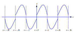
Figure 12.2.3 : The odd extension of a function that does not satisfy \ref{eq:12.2.13} 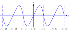
Figure 12.2.4 : The odd extension of a function that satisfies \ref{eq:12.2.13} (b) From Figure 12.2.5 ,
\[q'_-(2kL)=-h'_+(0)\quad \text{and} \quad q'_+(2kL)=h'_+(0),\nonumber\]
so \(q\) is differentiable at \(x=2kL\) if and only if \(h'_+(0)=0\). Also,
\[q'_-((2k-1)L)=h'_-(L) \quad \text{and} \quad q'_+((2k-1)L)= -h'_-(L) ,\nonumber\]
so \(q\) is differentiable at \(x=(2k-1)L\) if and only if \(h'_-(L)=0\). Therefore \(q\) is differentiable on \((-\infty,\infty)\) if and only if \(h'_{+}(0)=h'_\: (L)=0\), as in Figure 12.2.6 . This completes the proof.
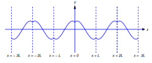
Figure 12.2.5 : The even extension of a function that doesn't satisfy \ref{eq:12.2.14} 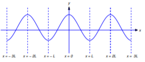
Figure 12.2.6 : The even extension of a function that satisfies \ref{eq:12.2.14}
The formal solution of \(\eqref{eq:12.2.1}\) is an actual solution if \(g\) is differentiable on \([0,L]\) and
\[\label{eq:12.2.15} g(0)=g(L)=0,\]
while \(f\) is twice differentiable on \([0,L]\) and
\[\label{eq:12.2.16} f(0)=f(L)=0\]
and
\[\label{eq:12.2.17} f''_+(0)=f''_-(L)=0.\]
- Proof
-
We first show that \(S_g\) is differentiable and \(S_f\) is twice differentiable on \((-\infty,\infty)\). We’ll then differentiate Equation \ref{eq:12.2.9} twice with respect to \(x\) and \(t\) and verify that Equation \ref{eq:12.2.9} is an actual solution of Equation \ref{eq:12.2.1}.
Since \(f\) and \(g\) are continuous on \((0,L)\), Theorem 11.3.2 implies that \(S_f(x)=f(x)\) and \(S_g(x)=g(x)\) on \([0,L]\). Therefore \(S_f\) and \(S_g\) are the odd periodic extensions of \(f\) and \(g\). Since \(f\) and \(g\) are differentiable on \([0,L]\), Equation \ref{eq:12.2.15}, Equation \ref{eq:12.2.16}, and Theorem 12.2.3 a imply that \(S_f\) and \(S_g\) are differentiable on \((-\infty,\infty)\).
Since \(S_f'(x)=f'(x)\) on \([0,L]\) (one-sided derivatives at the endpoints), and \(S_f'\) is even (the derivative of an odd function is even), \(S_f'\) is the even periodic extension of \(f'\). By assumption, \(f'\) is differentiable on \([0,L]\). Because of Equation \ref{eq:12.2.17}, Theorem 12.2.3 b with \(h=f'\) and \(q=S_f'\) implies that \(S_f''\) exists on \((-\infty,\infty)\).
Now we can differentiate Equation \ref{eq:12.2.9} twice with respect to \(x\) and \(t\):
\[u_x(x,t)={1\over2}[S_f'(x+at)+S_f'(x-at)]+ {1\over2a}[S_g(x+at)-S_g(x-at)],\nonumber\]
\[\label{eq:12.2.18} u_{xx}(x,t)={1\over2}[S_f''(x+at)+S_f''(x-at)]+ {1\over2a}[S_g'(x+at)-S_g'(x-at)],\]
\[\label{eq:12.2.19} u_t(x,t)={a\over2}[S_f'(x+at)-S_f'(x-at)]+ {1\over2}[S_g(x+at)+S_g(x-at)],\]
and
\[\label{eq:12.2.20} u_{tt}(x,t)={a^2\over2}[S_f''(x+at)-S_f''(x-at)]+ {a\over2}[S_g'(x+at)-S_g'(x-at)].\]
Comparing Equation \ref{eq:12.2.18} and Equation \ref{eq:12.2.20} shows that \(u_{tt}(x,t)=a^2u_{xx}(x,t)\) for all \((x,t)\).
From Equation \ref{eq:12.2.8}, \(u(0,t)=u(L,t)=0\) for all \(t\). From Equation \ref{eq:12.2.9}, \(u(x,0)=S_f(x)\) for all \(x\), and therefore, in particular,
\[u(x,0)=f(x),\quad 0\le x< L.\nonumber\]
From Equation \ref{eq:12.2.19}, \(u_t(x,0)=S_g(x)\) for all \(x\), and therefore, in particular,
\[u_t(x,0)=g(x),\quad 0\le x< L.\nonumber\]
Therefore \(u\) is an actual solution of Equation \ref{eq:12.2.1}. This completes the proof.
Equation \ref{eq:12.2.9} is called d’Alembert’s solution of Equation \ref{eq:12.2.1}. Although d’Alembert’s solution was useful for proving Theorem 12.2.4
and is very useful in a slightly different context (Exercises 12.2.63 - 12.2.68), Equation \ref{eq:12.2.8} is preferable for computational purposes.
Solve Equation \ref{eq:12.2.1} with
\[f(x)=x(x^3-2Lx^2+L^2) \quad \text{and} \quad g(x)=x(L-x).\nonumber \]
Solution
We leave it to you to verify that \(f\) and \(g\) satisfy the assumptions of Theorem 12.2.4 .
From Exercise 11.3.39,
\[S_f(x)={96L^4\over\pi^5}\sum_{n=1}^\infty{1\over(2n-1)^5}\sin{(2n-1)\pi x\over L}.\nonumber\]
From Exercise 11.3.36,
\[S_g(x)={8L^2\over\pi^3}\sum_{n=1}^\infty{1\over(2n-1)^3}\sin{(2n-1)\pi x\over L}.\nonumber\]
From Equation \ref{eq:12.2.8},
\[\begin{aligned} u(x, t)=& \frac{96 L^{4}}{\pi^{5}} \sum_{n=1}^{\infty} \frac{1}{(2 n-1)^{5}} \cos \frac{(2 n-1) \pi a t}{L} \sin \frac{(2 n-1) \pi x}{L} \\ &+\frac{8 L^{3}}{a \pi^{4}} \sum_{n=1}^{\infty} \frac{1}{(2 n-1)^{4}} \sin \frac{(2 n-1) \pi a t}{L} \sin \frac{(2 n-1) \pi x}{L} \end{aligned}\nonumber \]
Theorem 12.1.2 implies that \(u_{xx}\) and \(u_{tt}\) can be obtained by term by term differentiation, for all \((x,t)\), so \(u_{tt}=a^2u_{xx}\) for all \((x,t)\) (Exercise 12.2.62). Moreover, Theorem 11.3.2 implies that \(S_f(x)=f(x)\) and \(S_g(x)=g(x)\) if \(0\le x\le L\). Therefore \(u(x,0)=f(x)\) and \(u_t(x,0)=g(x)\) if \(0\le x\le L\). Hence, \(u\) is an actual solution of the initial-boundary value problem.
In solving a specific initial-boundary value problem (Equation \ref{eq:12.2.1}), it is convenient to solve the problem with \(g \equiv 0\), then with \(f \equiv 0\), and add the solutions to obtain the solution of the given problem. Because of this, either \(f \equiv 0\) or \(g \equiv 0\) in all the specific initial-boundary value problems in the exercises.
The Plucked String
If \(f\) and \(g\) don’t satisfy the assumptions of Theorem 12.2.4 , then Equation \ref{eq:12.2.8} is not an actual solution of Equation \ref{eq:12.2.1} in fact, it can be shown that Equation \ref{eq:12.2.1} doesn’t have an actual solution in this case. Nevertheless, \(u\) is defined for all \((x,t)\), and we can see from Equation \ref{eq:12.2.18} and Equation \ref{eq:12.2.20} that \(u_{tt}(x,t)=a^2u_{xx}(x,t)\) for all \((x,t)\) such that \(S_f''(x\pm at)\) and \(S_g'(x\pm at)\) exist. Moreover, \(u\) may still provide a useful approximation to the vibration of the string; a laboratory experiment can confirm or deny this.
We’ll now consider the initial-boundary value problem Equation \ref{eq:12.2.1} with
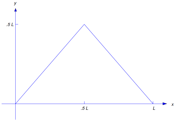
\[\label{eq:12.2.21} f(x)= \left\{\begin{array}{cl} x,&0\le x\le{L\over2},\\L-x,&{L\over2}\le x\le L \end{array}\right.\]
and \(g\equiv0\). Since \(f\) is not differentiable at \(x=L/2\), it does’nt satisfy the assumptions of Theorem 12.2.4 , so the formal solution of Equation \ref{eq:12.2.1} can’t be an actual solution. Nevertheless, it is instructive to investigate the properties of the formal solution.
The graph of \(f\) is shown in Figure 12.2.7 . Intuitively, we are plucking the string by half its length at the middle. You’re right if you think this is an extraordinarily large displacement; however, we could remove this objection by multiplying the function in Figure 12.2.7 by a small constant. Since this would just multiply the formal solution by the same constant, we’ll leave \(f\) as we’ve defined it. Similar comments apply to the exercises.
From Exercise 11.3.15, the Fourier sine series of \(f\) on \([0,L]\) is
\[S_{f}(x)=\frac{4 L}{\pi^{2}} \sum_{n=1}^{\infty} \frac{(-1)^{n+1}}{(2 n-1)^{2}} \sin \frac{(2 n-1) \pi x}{L}\nonumber\]
which converges to \(f\) for all \(x\) in \([0,L]\), by Theorem 11.3.2. Therefore
\[\label{eq:12.2.22} u(x, t)=\frac{4 L}{\pi^{2}} \sum_{n=1}^{\infty} \frac{(-1)^{n+1}}{(2 n-1)^{2}} \cos \frac{(2 n-1) \pi a t}{L} \sin \frac{(2 n-1) \pi x}{L}\]
This series converges absolutely for all \((x,t)\) by the comparison test, since the series
\[\sum_{n=1}^\infty{1\over(2n-1)^2}\nonumber\]
converges. Moreover, Equation \ref{eq:12.2.22} satisfies the boundary conditions
\[u(0,t)=u(L,t)=0,\quad t>0,\nonumber\]
and the initial condition
\[u(x,0)=f(x),\quad 0\le x\le L.\nonumber\]
However, we can’t justify differentiating Equation \ref{eq:12.2.22} term by term even once, and formally differentiating it twice term by term produces a series that diverges for all \((x,t)\). (Verify.). Therefore we use d’Alembert’s form
\[\label{eq:12.2.23} u(x,t)={1\over2}[S_f(x+at)+S_f(x-at)]\]
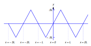
for \(u\) to study its derivatives. Figure 12.2.8 shows the graph of \(S_f\), which is the odd periodic extension of \(f\). You can see from the graph that \(S_f\) is differentiable at \(x\) (and \(S_f'(x)=\pm1\)) if and only if \(x\) is not an odd multiple of \(L/2\).
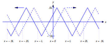
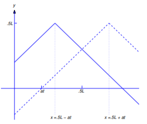
In Figure 12.2.9 the dashed and solid curves are the graphs of \(y=S_f(x-at)\) and \(y=S_f(x+at)\) respectively, for a fixed value of \(t\). As \(t\) increases the dashed curve moves to the right and the solid curve moves to the left. For this reason, we say that the functions \(u_1(x,t)=S_f(x+at)\) and \(u_2(x,t)=S_f(x-at)\) are traveling waves. Note that \(u_1\) satisfies the wave equation at \((x,t)\) if \(x+at\) is not an odd multiple of \(L/2\) and \(u_2\) satisfies the wave equation at \((x,t)\) if \(x-at\) is not an odd multiple of \(L/2\). Therefore Equation \ref{eq:12.2.23} (or, equivalently, Equation \ref{eq:12.2.22}) satisfies \(u_{tt}(x,t)=a^2u_{xx}(x,t)=0\) for all \((x,t)\) such that neither \(x-at\) nor \(x+at\) is an odd multiple of \(L/2\).
We conclude by finding an explicit formula for \(u(x,t)\) under the assumption that
\[\label{eq:12.2.24} 0\le x\le L\quad \text{and} \quad 0\le t\le L/2a.\]
To see how this formula can be used to compute \(u(x,t)\) for \(0\le x\le L\) and arbitrary \(t\), we refer you to Exercise 12.2.16.
From Figure 12.2.10 ,
\[S_f(x-at)= \left\{\begin{array}{cl} x-at,&0\le x\le {L\over2}+at,\\[4pt] L-x+at,&{L\over2}+at\le x\le L \end{array}\right.\nonumber\]
and
\[S_f(x+at)= \left\{\begin{array}{cl} x+at,&0\le x\le {L\over2}-at,\\[4pt] L-x-at,&{L\over2}-at\le x\le L \end{array}\right.\nonumber\]
if \((x,t)\) satisfies Equation \ref{eq:12.2.24}.
Therefore, from Equation \ref{eq:12.2.23},
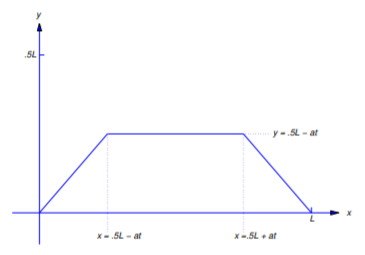
\[u(x,t)= \left\{\begin{array}{cl} x,&0\le x\le{L\over2}-at,\\[4pt] {L\over2}-at,&{L\over2}-at\le x\le{L\over2}+at,\\[4pt] L-x,&{L\over2}-at\le x\le L \end{array}\right.\nonumber\]
if \((x,t)\) satisfies Equation \ref{eq:12.2.24}. Figure 12.2.11 is the graph of this function on \([0,L]\) for a fixed \(t\) in \((0,L/2a)\).
Using Technology
Although the formal solution
\[u(x,t)=\sum_{n=1}^\infty\left(\alpha_n\cos{n\pi at\over L}+{\beta_nL\over n\pi a}\sin{n\pi at\over L}\right) \sin{n\pi x\over L}\nonumber\]
of Equation \ref{eq:12.2.1} is defined for all \((x,t)\), we are mainly interested in its behavior for \(0\le x\le L\) and \(t\ge0\). In fact, it is sufficient to consider only values of \(t\) in the interval \(0\le t<2L/a\), since
\[u(x,t+2kL/a)=u(x,t)\nonumber\]
for all \((x,t)\) if \(k\) is an integer. (Verify.)
You can create an animation of the motion of the string by performing the following numerical experiment.
Let \(m\) and \(k\) be positive integers. Let
\[t_j={2Lj\over ka},\quad j=0,1,\dots k;\nonumber\]
thus, \(t_0\), \(t_1\), …\(t_k\) are equally spaced points in \([0,2L/a]\). For each \(j=0\), \(1\),\(2\), …\(k\), graph the partial sum
\[u_m(x,t_j)=\sum_{n=1}^m\left(\alpha_n\cos{n\pi at_j\over L}+{\beta_nL\over n\pi a}\sin{n\pi at_j\over L}\right) \sin{n\pi x\over L}\nonumber\]
on \([0,L]\) as a function of \(x\). Write your program so that each graph remains displayed on the monitor for a short time, and is then deleted and replaced by the next. Repeat this procedure for various values of \(m\) and \(k\).


