
7.0: Prelude to Green's Functions and Nonhomogeneous Problems
- Page ID
- 105971
"The young theoretical physicists of a generation or two earlier subscribed to the belief that: If you haven’t done something important by age 30, you never will. Obviously, they were unfamiliar with the history of George Green, the miller of Nottingham." - Julian Schwinger (1918-1994)
The wave equation, heat equation, and Laplace's equation are typical homogeneous partial differential equations. They can be written in the form \[\mathcal{L} u(x)=0,\nonumber \] where \(\mathcal{L}\) is a differential operator. For example, these equations can be written as \[\begin{align} \left(\frac{\partial^{2}}{\partial t^{2}}-c^{2} \nabla^{2}\right) u &=0,\nonumber \\ \left(\frac{\partial}{\partial t}-k \nabla^{2}\right) u &=0,\nonumber \\ \nabla^{2} u &=0 .\label{eq:1} \end{align}\]
In this chapter we will explore solutions of nonhomogeneous partial differential equations, \[\mathcal{L} u(x)=f(x),\nonumber \] by seeking out the so-called Green’s function. The history of the Green’s function dates back to 1828, when George Green published work in which he sought solutions of Poisson’s equation \(\nabla^{2} u=f\) for the electric potential \(u\) defined inside a bounded volume with specified boundary conditions on the surface of the volume. He introduced a function now identified as what Riemann later coined the "Green’s function". In this chapter we will derive the initial value Green’s function for ordinary differential equations. Later in the chapter we will return to boundary value Green’s functions and Green’s functions for partial differential equations.
George Green (1793-1841), a British mathematical physicist who had little formal education and worked as a miller and a baker, published An Essay on the Application of Mathematical Analysis to the Theories of Electricity and Magnetism in which he not only introduced what is now known as Green’s function, but he also introduced potential theory and Green’s Theorem in his studies of electricity and magnetism. Recently his paper was posted at arXiv.org, arXiv:o807.0088.
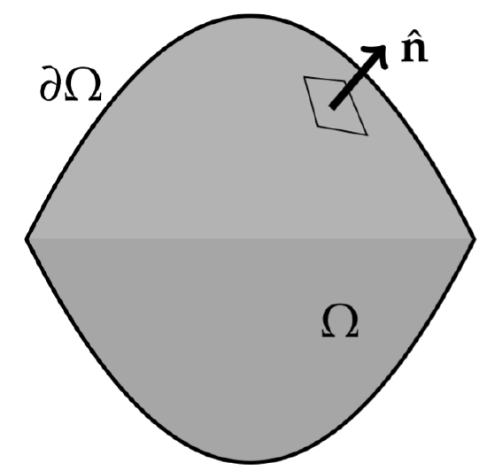
As a simple example, consider Poisson’s equation, \[\nabla^2 u(\mathbf{r})=f(\mathbf{r}).\nonumber\] Let Poisson’s equation hold inside a region \(\Omega\) bounded by the surface \(\partial \Omega\) as shown in Figure \(\PageIndex{1}\). This is the nonhomogeneous form of Laplace’s equation. The nonhomogeneous term, \(f(\mathbf{r})\), could represent a heat source in a steady-state problem or a charge distribution (source) in an electrostatic problem.
Now think of the source as a point source in which we are interested in the response of the system to this point source. If the point source is located at a point \(\mathbf{r}^{\prime}\), then the response to the point source could be felt at points r. We will call this response \(G\left(\mathbf{r}, \mathbf{r}^{\prime}\right)\). The response function would satisfy a point source equation of the form \[\nabla^{2} G\left(\mathbf{r}, \mathbf{r}^{\prime}\right)=\delta\left(\mathbf{r}-\mathbf{r}^{\prime}\right) \text {. }\nonumber \] Here \(\delta\left(\mathbf{r}-\mathbf{r}^{\prime}\right)\) is the Dirac delta function, which we will consider in more detail in Section 9.4. A key property of this generalized function is the sifting property, \[\int_{\Omega} \delta\left(\mathbf{r}-\mathbf{r}^{\prime}\right) f(\mathbf{r}) d V=f\left(\mathbf{r}^{\prime}\right) .\nonumber \]
The connection between the Green’s function and the solution to Poisson’s equation can be found from Green’s second identity: \[\int_{\partial \Omega}[\phi \nabla \psi-\psi \nabla \phi] \cdot \mathbf{n} d S=\int_{\Omega}\left[\phi \nabla^{2} \psi-\psi \nabla^{2} \phi\right] d V .\nonumber \] Letting \(\phi=u(\mathbf{r})\) and \(\psi=G\left(\mathbf{r}, \mathbf{r}^{\prime}\right)\), we have\(^{1}\) \[\begin{align} & \int_{\partial \Omega}\left[u(\mathbf{r}) \nabla G\left(\mathbf{r}, \mathbf{r}^{\prime}\right)-G\left(\mathbf{r}, \mathbf{r}^{\prime}\right) \nabla u(\mathbf{r})\right] \cdot \mathbf{n} d S\nonumber \\ =& \int_{\Omega}\left[u(\mathbf{r}) \nabla^{2} G\left(\mathbf{r}, \mathbf{r}^{\prime}\right)-G\left(\mathbf{r}, \mathbf{r}^{\prime}\right) \nabla^{2} u(\mathbf{r})\right] d V\nonumber \\ =& \int_{\Omega}\left[u(\mathbf{r}) \delta\left(\mathbf{r}-\mathbf{r}^{\prime}\right)-G\left(\mathbf{r}, \mathbf{r}^{\prime}\right) f(\mathbf{r})\right] d V\nonumber \\ =& u\left(\mathbf{r}^{\prime}\right)-\int_{\Omega} G\left(\mathbf{r}, \mathbf{r}^{\prime}\right) f(\mathbf{r}) d V .\label{eq:2} \end{align}\] Solving for \(u\left(\mathbf{r}^{\prime}\right)\), we have \[\begin{align} u\left(\mathbf{r}^{\prime}\right)=& \int_{\Omega} G\left(\mathbf{r}, \mathbf{r}^{\prime}\right) f(\mathbf{r}) d V\nonumber \\ &+\int_{\partial \Omega}\left[u(\mathbf{r}) \nabla G\left(\mathbf{r}, \mathbf{r}^{\prime}\right)-G\left(\mathbf{r}, \mathbf{r}^{\prime}\right) \nabla u(\mathbf{r})\right] \cdot \mathbf{n} d S .\label{eq:3} \end{align}\] If both \(u(\mathbf{r})\) and \(G\left(\mathbf{r}, \mathbf{r}^{\prime}\right)\) satisfied Dirichlet conditions, \(u=0\) on \(\partial \Omega\), then the last integral vanishes and we are left with\(^{2}\) \[u\left(\mathbf{r}^{\prime}\right)=\int_{\Omega} G\left(\mathbf{r}, \mathbf{r}^{\prime}\right) f(\mathbf{r}) d V .\nonumber \]
In many applications there is a symmetry, \[G\left(\mathbf{r}, \mathbf{r}^{\prime}\right)=G\left(\mathbf{r}^{\prime}, \mathbf{r}\right)\nonumber \] Then, the result can be written as \[u(\mathbf{r})=\int_{\Omega} G\left(\mathbf{r}, \mathbf{r}^{\prime}\right) f\left(\mathbf{r}^{\prime}\right) d V^{\prime} .\nonumber \]
So, if we know the Green’s function, we can solve the nonhomogeneous differential equation. In fact, we can use the Green’s function to solve nonhomogenous boundary value and initial value problems. That is what we will see develop in this chapter as we explore nonhomogeneous problems in more detail. We will begin with the search for Green’s functions for ordinary differential equations.