11.3: Hyperbolic Functions

So, are there any other functions that are useful in physics? Actually, there are many more. However, you have probably not see many of them to date. We will see by the end of the semester that there are many important functions that arise as solutions of some fairly generic, but important, physics problems. In your calculus classes you have also seen that some relations are represented in parametric form. However, there is at least one other set of elementary functions, which you should already know about. These are the hyperbolic functions. Such functions are useful in representing hanging cables, unbounded orbits, and special traveling waves called solitons. They also play a role in special and general relativity.

Solitons

Solitons are special solutions to some generic nonlinear wave equations. They typically experience elastic collisions and play special roles in a variety of fields in physics, such as hydrodynamics and optics. A simple soliton solution is of the form \[u(x, t)=2 \eta^{2} \operatorname{sech}^{2} \eta\left(x-4 \eta^{2} t\right) .\nonumber \]

Note

We will later see the connection between the hyperbolic and trigonometric functions in Chapter 8.

Figure \(\PageIndex{1}\): Plots of \(\operatorname{cosh}x\) and \(\operatorname{sinh}x\). Note that \(\operatorname{sinh}0=0\), \(\operatorname{cosh}0=1\), and \(\operatorname{cosh}x\geq 1\).

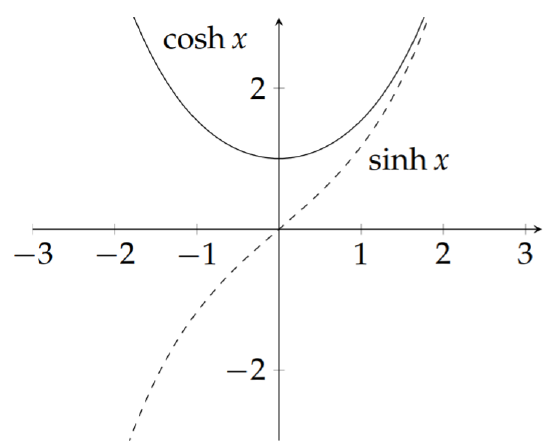
Hyperbolic functions are actually related to the trigonometric functions, as we shall see after a little bit of complex function theory. For now, we just want to recall a few definitions and identities. Just as all of the trigonometric functions can be built from the sine and the cosine, the hyperbolic functions can be defined in terms of the hyperbolic sine and hyperbolic cosine (shown in Figure \(\PageIndex{1}\)):

\[\begin{align}\operatorname{sinh}x&=\frac{e^x-e^{-x}}{2},\label{eq:1} \\[4pt] \operatorname{\cosh}x&=\frac{e^x+e^{-x}}{2}.\label{eq:2}\end{align}\] There are four other hyperbolic functions. These are defined in terms of the above functions similar to the relations between the trigonometric functions. We have \[\begin{align} &\operatorname{tanh} x=\frac{1}{\cosh x}=\frac{2}{e^x+e^{-x}},\label{eq:3}\\[4pt] &\operatorname{sech} x=\frac{1}{\cosh x}=\frac{2}{e^{x}+e^{-x}},\label{eq:4} \\[4pt] &\operatorname{csch} x=\frac{1}{\sinh x}=\frac{2}{e^{x}-e^{-x}},\label{eq:5} \\[4pt] &\operatorname{coth} x=\frac{1}{\tanh x}=\frac{e^{x}+e^{-x}}{e^{x}-e^{-x}} .\label{eq:6} \end{align}\]

There are also a whole set of identities, similar to those for the trigonometric functions. For example, the Pythagorean identity for trigonometric functions, \(\sin ^{2} \theta+\cos ^{2} \theta=1\), is replaced by the identity \[\cosh ^{2} x-\sinh ^{2} x=1 .\nonumber \] This is easily shown by simply using the definitions of these functions. This identity is also useful for providing a parametric set of equations describing hyperbolae. Letting \(x=a \cosh t\) and \(y=b \sinh t\), one has \[\frac{x^{2}}{a^{2}}-\frac{y^{2}}{b^{2}}=\cosh ^{2} t-\sinh ^{2} t=1 .\nonumber \]

A list of commonly needed hyperbolic function identities are given by the following: \[\begin{align} \cosh ^{2} x-\sinh ^{2} x &=1, & \label{eq:7} \\[4pt] \tanh ^{2} x+\operatorname{sech}^{2} x &=1, \label{eq:8} \\[4pt] \cosh (A \pm B) &=\cosh A \cosh B \pm \sinh A \sinh B, \label{eq:9} \\[4pt] \sinh (A \pm B) &=\sinh A \cosh B \pm \sinh B \cosh A, \label{eq:10} \\[4pt] \cosh 2 x &=\cosh ^{2} x+\sinh ^{2} x,\label{eq:11} \\[4pt] \sinh 2 x &=2 \sinh x \cosh x,\label{eq:12} \\[4pt] \cosh ^{2} x &=\frac{1}{2}(1+\cosh 2 x),\label{eq:13} \\[4pt] \sinh ^{2} x &=\frac{1}{2}(\cosh 2 x-1) .\label{eq:14} \end{align}\] Note the similarity with the trigonometric identities. Other identities can be derived from these.

There also exist inverse hyperbolic functions and these can be written in terms of logarithms. As with the inverse trigonometric functions, we begin with the definition \[y=\sinh ^{-1} x \quad \Leftrightarrow \quad x=\sinh y .\label{eq:15}\] The aim is to write \(y\) in terms of \(x\) without using the inverse function. First, we note that \[x=\frac{1}{2}\left(e^{y}-e^{-y}\right) .\label{eq:16}\] Next we solve for \(e^{y}\). This is done by noting that \(e^{-y}=\frac{1}{e^{y}}\) and rewriting the previous equation as \[0=\left(e^{y}\right)^{2}-2 x e^{y}-1 .\label{eq:17}\] This equation is in quadratic form which we can solve using the quadratic formula as \[e^{y}=x+\sqrt{1+x^{2}} .\nonumber \] (There is only one root as we expect the exponential to be positive.)

The final step is to solve for \(y\), \[y=\ln \left(x+\sqrt{1+x^{2}}\right) .\label{eq:18}\]

Inverse Hyperbolic Functions

The inverse hyperbolic functions are given by \[\begin{aligned} \sinh ^{-1} x &=\ln \left(x+\sqrt{1+x^{2}}\right) \\[4pt] \cosh ^{-1} x &=\ln \left(x+\sqrt{x^{2}-1}\right) \\[4pt] \tanh ^{-1} x &=\frac{1}{2} \ln \frac{1+x}{1-x} \end{aligned}\]