
11.7: Power Series
- Page ID
- 91031

\( \newcommand{\vecs}[1]{\overset { \scriptstyle \rightharpoonup} {\mathbf{#1}} } \)
\( \newcommand{\vecd}[1]{\overset{-\!-\!\rightharpoonup}{\vphantom{a}\smash {#1}}} \)
\( \newcommand{\dsum}{\displaystyle\sum\limits} \)
\( \newcommand{\dint}{\displaystyle\int\limits} \)
\( \newcommand{\dlim}{\displaystyle\lim\limits} \)
\( \newcommand{\id}{\mathrm{id}}\) \( \newcommand{\Span}{\mathrm{span}}\)
( \newcommand{\kernel}{\mathrm{null}\,}\) \( \newcommand{\range}{\mathrm{range}\,}\)
\( \newcommand{\RealPart}{\mathrm{Re}}\) \( \newcommand{\ImaginaryPart}{\mathrm{Im}}\)
\( \newcommand{\Argument}{\mathrm{Arg}}\) \( \newcommand{\norm}[1]{\| #1 \|}\)
\( \newcommand{\inner}[2]{\langle #1, #2 \rangle}\)
\( \newcommand{\Span}{\mathrm{span}}\)
\( \newcommand{\id}{\mathrm{id}}\)
\( \newcommand{\Span}{\mathrm{span}}\)
\( \newcommand{\kernel}{\mathrm{null}\,}\)
\( \newcommand{\range}{\mathrm{range}\,}\)
\( \newcommand{\RealPart}{\mathrm{Re}}\)
\( \newcommand{\ImaginaryPart}{\mathrm{Im}}\)
\( \newcommand{\Argument}{\mathrm{Arg}}\)
\( \newcommand{\norm}[1]{\| #1 \|}\)
\( \newcommand{\inner}[2]{\langle #1, #2 \rangle}\)
\( \newcommand{\Span}{\mathrm{span}}\) \( \newcommand{\AA}{\unicode[.8,0]{x212B}}\)
\( \newcommand{\vectorA}[1]{\vec{#1}} % arrow\)
\( \newcommand{\vectorAt}[1]{\vec{\text{#1}}} % arrow\)
\( \newcommand{\vectorB}[1]{\overset { \scriptstyle \rightharpoonup} {\mathbf{#1}} } \)
\( \newcommand{\vectorC}[1]{\textbf{#1}} \)
\( \newcommand{\vectorD}[1]{\overrightarrow{#1}} \)
\( \newcommand{\vectorDt}[1]{\overrightarrow{\text{#1}}} \)
\( \newcommand{\vectE}[1]{\overset{-\!-\!\rightharpoonup}{\vphantom{a}\smash{\mathbf {#1}}}} \)
\( \newcommand{\vecs}[1]{\overset { \scriptstyle \rightharpoonup} {\mathbf{#1}} } \)
\(\newcommand{\longvect}{\overrightarrow}\)
\( \newcommand{\vecd}[1]{\overset{-\!-\!\rightharpoonup}{\vphantom{a}\smash {#1}}} \)
\(\newcommand{\avec}{\mathbf a}\) \(\newcommand{\bvec}{\mathbf b}\) \(\newcommand{\cvec}{\mathbf c}\) \(\newcommand{\dvec}{\mathbf d}\) \(\newcommand{\dtil}{\widetilde{\mathbf d}}\) \(\newcommand{\evec}{\mathbf e}\) \(\newcommand{\fvec}{\mathbf f}\) \(\newcommand{\nvec}{\mathbf n}\) \(\newcommand{\pvec}{\mathbf p}\) \(\newcommand{\qvec}{\mathbf q}\) \(\newcommand{\svec}{\mathbf s}\) \(\newcommand{\tvec}{\mathbf t}\) \(\newcommand{\uvec}{\mathbf u}\) \(\newcommand{\vvec}{\mathbf v}\) \(\newcommand{\wvec}{\mathbf w}\) \(\newcommand{\xvec}{\mathbf x}\) \(\newcommand{\yvec}{\mathbf y}\) \(\newcommand{\zvec}{\mathbf z}\) \(\newcommand{\rvec}{\mathbf r}\) \(\newcommand{\mvec}{\mathbf m}\) \(\newcommand{\zerovec}{\mathbf 0}\) \(\newcommand{\onevec}{\mathbf 1}\) \(\newcommand{\real}{\mathbb R}\) \(\newcommand{\twovec}[2]{\left[\begin{array}{r}#1 \\ #2 \end{array}\right]}\) \(\newcommand{\ctwovec}[2]{\left[\begin{array}{c}#1 \\ #2 \end{array}\right]}\) \(\newcommand{\threevec}[3]{\left[\begin{array}{r}#1 \\ #2 \\ #3 \end{array}\right]}\) \(\newcommand{\cthreevec}[3]{\left[\begin{array}{c}#1 \\ #2 \\ #3 \end{array}\right]}\) \(\newcommand{\fourvec}[4]{\left[\begin{array}{r}#1 \\ #2 \\ #3 \\ #4 \end{array}\right]}\) \(\newcommand{\cfourvec}[4]{\left[\begin{array}{c}#1 \\ #2 \\ #3 \\ #4 \end{array}\right]}\) \(\newcommand{\fivevec}[5]{\left[\begin{array}{r}#1 \\ #2 \\ #3 \\ #4 \\ #5 \\ \end{array}\right]}\) \(\newcommand{\cfivevec}[5]{\left[\begin{array}{c}#1 \\ #2 \\ #3 \\ #4 \\ #5 \\ \end{array}\right]}\) \(\newcommand{\mattwo}[4]{\left[\begin{array}{rr}#1 \amp #2 \\ #3 \amp #4 \\ \end{array}\right]}\) \(\newcommand{\laspan}[1]{\text{Span}\{#1\}}\) \(\newcommand{\bcal}{\cal B}\) \(\newcommand{\ccal}{\cal C}\) \(\newcommand{\scal}{\cal S}\) \(\newcommand{\wcal}{\cal W}\) \(\newcommand{\ecal}{\cal E}\) \(\newcommand{\coords}[2]{\left\{#1\right\}_{#2}}\) \(\newcommand{\gray}[1]{\color{gray}{#1}}\) \(\newcommand{\lgray}[1]{\color{lightgray}{#1}}\) \(\newcommand{\rank}{\operatorname{rank}}\) \(\newcommand{\row}{\text{Row}}\) \(\newcommand{\col}{\text{Col}}\) \(\renewcommand{\row}{\text{Row}}\) \(\newcommand{\nul}{\text{Nul}}\) \(\newcommand{\var}{\text{Var}}\) \(\newcommand{\corr}{\text{corr}}\) \(\newcommand{\len}[1]{\left|#1\right|}\) \(\newcommand{\bbar}{\overline{\bvec}}\) \(\newcommand{\bhat}{\widehat{\bvec}}\) \(\newcommand{\bperp}{\bvec^\perp}\) \(\newcommand{\xhat}{\widehat{\xvec}}\) \(\newcommand{\vhat}{\widehat{\vvec}}\) \(\newcommand{\uhat}{\widehat{\uvec}}\) \(\newcommand{\what}{\widehat{\wvec}}\) \(\newcommand{\Sighat}{\widehat{\Sigma}}\) \(\newcommand{\lt}{<}\) \(\newcommand{\gt}{>}\) \(\newcommand{\amp}{&}\) \(\definecolor{fillinmathshade}{gray}{0.9}\)Another example of an infinite series that the student has encountered in previous courses is the power series. Examples of such series are provided by Taylor and Maclaurin series.
Actually, what are now known as Taylor and Maclaurin series were known long before they were named. James Gregory (1638-1675) has been recognized for discovering Taylor series, which were later named after Brook Taylor (1685-1731). Similarly, Colin Maclaurin (1698-1746) did not actually discover Maclaurin series, but the name was adopted because of his particular use of series.
A power series expansion about \(x=a\) with coefficient sequence \(c_{n}\) is given by \(\sum_{n=0}^{\infty} c_{n}(x-a)^{n}\). For now we will consider all constants to be real numbers with \(x\) in some subset of the set of real numbers.
Consider the following expansion about \(x=0\) : \[\sum_{n=0}^{\infty} x^{n}=1+x+x^{2}+\ldots\label{eq:1}\]
We would like to make sense of such expansions. For what values of \(x\) will this infinite series converge? Until now we did not pay much attention to which infinite series might converge. However, this particular series is already familiar to us. It is a geometric series. Note that each term is gotten from the previous one through multiplication by \(r=x\). The first term is \(a=1\). So, from Equation (11.6.6), we have that the sum of the series is given by \[\sum\limits_{n=0}^\infty x^n=\frac{1}{1-x},\quad |x|<1.\nonumber\]
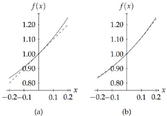
In this case we see that the sum, when it exists, is a simple function. In fact, when \(x\) is small, we can use this infinite series to provide approximations to the function \((1 − x)^{−1}\). If \(x\) is small enough, we can write \[(1-x)^{-1}\approx 1+x.\nonumber\] In Figure \(\PageIndex{1}\)(a) we see that for small values of \(x\) these functions do agree.
Of course, if we want better agreement, we select more terms. In Figure \(\PageIndex{1}\)(b) we see what happens when we do so. The agreement is much better. But extending the interval, we see in Figure \(\PageIndex{2}\) that keeping only quadratic terms may not be good enough. Keeping the cubic terms gives better agreement over the interval.

Finally, in Figure \(\PageIndex{3}\) we show the sum of the first 21 terms over the entire interval \([-1,1]\). Note that there are problems with approximations near the endpoints of the interval, \(x=\pm 1\).

Such polynomial approximations are called Taylor polynomials. Thus, \(T_{3}(x)=1+x+x^{2}+x^{3}\) is the third order Taylor polynomial approximation of \(f(x)=\frac{1}{1-x}\).
With this example we have seen how useful a series representation might be for a given function. However, the series representation was a simple geometric series, which we already knew how to sum. Is there a way to begin with a function and then find its series representation? Once we have such a representation, will the series converge to the function with which we started? For what values of \(x\) will it converge? These questions can be answered by recalling the definitions of Taylor and Maclaurin series.
A Taylor series expansion of \(f(x)\) about \(x=a\) is the series \[f(x) \sim \sum_{n=0}^{\infty} c_{n}(x-a)^{n},\label{eq:2}\] where \[c_{n}=\frac{f^{(n)}(a)}{n !} .\label{eq:3}\]
Note that we use \(\sim\) to indicate that we have yet to determine when the series may converge to the given function. A special class of series are those Taylor series for which the expansion is about \(x=0\). These are called Maclaurin series.
A Maclaurin series expansion of \(f(x)\) is a Taylor series expansion of \(f(x)\) about \(x=0\), or \[f(x) \sim \sum_{n=0}^{\infty} c_{n} x^{n},\label{eq:4} \] where \[c_{n}=\frac{f^{(n)}(0)}{n !} .\label{eq:5}\]
Expand \(f(x)=e^{x}\) about \(x=0\).
Solution
We begin by creating a table. In order to compute the expansion coefficients, \(c_{n}\), we will need to perform repeated differentiations of \(f(x)\). So, we provide a table for these derivatives. Then, we only need to evaluate the second column at \(x=0\) and divide by \(n !\).
Table \(\PageIndex{1}\)
| \(n\) | \(f^{(n)}(x)\) | \(f^{(n)}(0)\) | \(c_{n}\) |
|---|---|---|---|
| 0 | \(e^{x}\) | \(e^{0}=1\) | \(\frac{1}{0 !}=1\) |
| 1 | \(e^{x}\) | \(e^{0}=1\) | \(\frac{1}{1 !}=1\) |
| 2 | \(e^{x}\) | \(e^{0}=1\) | \(\frac{1}{2 !}\) |
| 3 | \(e^{x}\) | \(e^{0}=1\) | \(\frac{1}{3 !}\) |
Next, we look at the last column and try to determine a pattern so that we can write down the general term of the series. If there is only a need to get a polynomial approximation, then the first few terms may be sufficient. In this case, the pattern is obvious: \(c_{n}=\frac{1}{n !}\). So, \[e^{x} \sim \sum_{n=0}^{\infty} \frac{x^{n}}{n !} .\nonumber \]
Expand \(f(x)=e^{x}\) about \(x=1\).
Solution
Here we seek an expansion of the form \(e^{x} \sim \sum_{n=0}^{\infty} c_{n}(x-1)^{n}\). We could create a table like the last example. In fact, the last column would have values of the form \(\frac{e}{v 1}\). (You should confirm this.) However, we will make use of the Maclaurin series expansion for \(e^{x}\) and get the result quicker. Note that \(e^{x}=e^{x-1+1}=e e^{x-1}\). Now, apply the known expansion for \(e^{x}\) : \[e^{x} \sim e\left(1+(x-1)+\frac{(x-1)^{2}}{2}+\frac{(x-1)^{3}}{3 !}+\ldots\right)=\sum_{n=0}^{\infty} \frac{e(x-1)^{n}}{n !}\nonumber \]
Expand \(f(x)=\frac{1}{1-x}\) about \(x=0\).
Solution
This is the example with which we started our discussion. We can set up a table in order to find the Maclaurin series coefficients. We see from the last column of the table that we get back the geometric series \(\eqref{eq:1}\).
Table \(\PageIndex{2}\)
| \(n\) | \(f^{(n)}(x)\) | \(f^{(n)}(0)\) | \(c_{n}\) |
|---|---|---|---|
| 0 | \(\frac{1}{1-x}\) | 1 | \(\frac{1}{0 !}=1\) |
| 1 | \(\frac{1}{(1-x)^{2}}\) | 1 | \(\frac{1}{1 !}=1\) |
| 2 | \(\frac{2(1)}{(1-x)^{3}}\) | \(2(1)\) | \(\frac{2 !}{2 !}=1\) |
| 3 | \(\frac{3(2)(1)}{(1-x)^{4}}\) | \(3(2)(1)\) | \(\frac{3 !}{3 !}=1\) |
So, we have found \[\frac{1}{1-x} \sim \sum_{n=0}^{\infty} x^{n} .\nonumber \]
We can replace \(\sim\) by equality if we can determine the range of \(x\)-values for which the resulting infinite series converges. We will investigate such convergence shortly.
Series expansions for many elementary functions arise in a variety of applications. Some common expansions are provided in Table \(\PageIndex{3}\).
We still need to determine the values of \(x\) for which a given power series converges. The first five of the above expansions converge for all reals, but the others only converge for \(|x|<1\).
We consider the convergence of \(\sum_{n=0}^{\infty} c_{n}(x-a)^{n}\). For \(x=a\) the series obviously converges. Will it converge for other points? One can prove
If \(\sum_{n=0}^{\infty} c_{n}(b-a)^{n}\) converges for \(b \neq a\), then \(\sum_{n=0}^{\infty} c_{n}(x-a)^{n}\) converges absolutely for all \(x\) satisfying \(|x-a|<|b-a|\).
This leads to three possibilities
- \(\sum_{n=0}^{\infty} c_{n}(x-a)^{n}\) may only converge at \(x=a\).
- \(\sum_{n=0}^{\infty} c_{n}(x-a)^{n}\) may converge for all real numbers.
- \(\sum_{n=0}^{\infty} c_{n}(x-a)^{n}\) converges for \(|x-a|<R\) and diverges for \(\mid x-\) \(a \mid>R\).
The number \(R\) is called the radius of convergence of the power series and \((a-R, a+R)\) is called the interval of convergence. Convergence at the endpoints of this interval has to be tested for each power series.
Table \(\PageIndex{3}\): Common Mclaurin Series Expansions
| Series Expansions You Should Know | ||
|---|---|---|
| \(e^{x}\) | \(=1+x+\frac{x^{2}}{2}+\frac{x^{3}}{3 !}+\frac{x^{4}}{4 !}+\ldots\) | \(=\sum_{n=0}^{\infty} \frac{x^{n}}{n !}\) |
| \(\cos \mathrm{x}\) | \(=1-\frac{x^{2}}{2}+\frac{x^{4}}{4 !}-\ldots\) | \(=\sum_{n=0}^{\infty}(-1)^{n} \frac{x^{2 n}}{(2 n) !}\) |
| \(\sin x\) | \(=x-\frac{x^{3}}{3 !}+\frac{x^{5}}{5 !}-\ldots\) | \(=\sum_{n=0}^{\infty}(-1)^{n} \frac{x^{2 n+1}}{(2 n+1) !}\) |
| \(\cosh x\) | \(=1+\frac{x^{2}}{2}+\frac{x^{4}}{4 !}+\ldots\) | \(=\sum_{n=0}^{\infty} \frac{x^{2 n}}{(2 n) !}\) |
| \(\sinh x\) | \(=x+\frac{x^{3}}{3 !}+\frac{x^{5}}{5 !}+\ldots\) | \(=\sum_{n=0}^{\infty} \frac{x^{2 n+1}}{(2 n+1) !}\) |
| \(\frac{1}{1-x}\) | \(=1+x+x^{2}+x^{3}+\ldots\) | \(=\sum_{n=0}^{\infty} x^{n}\) |
| \(\frac{1}{1+x}\) | \(=1-x+x^{2}-x^{3}+\ldots\) | \(=\sum_{n=0}^{\infty}(-x)^{n}\) |
| \(\tan ^{-1} x\) | \(=x-\frac{x^{3}}{3}+\frac{x^{5}}{5}-\frac{x^{7}}{7}+\ldots\) | \(=\sum_{n=0}^{\infty}(-1)^{n} \frac{x^{2 n+1}}{2 n+1}\) |
| \(\ln (1+x)\) | \(=x-\frac{x^{2}}{2}+\frac{x^{3}}{3}-\ldots\) | \(=\sum_{n=1}^{\infty}(-1)^{n+1} \frac{x^{n}}{n}\) |
In order to determine the interval of convergence, one needs only note that when a power series converges, it does so absolutely. So, we need only test the convergence of \(\sum_{n=0}^{\infty}\left|c_{n}(x-a)^{n}\right|=\sum_{n=0}^{\infty}\left|c_{n}\right||x-a|^{n}\). This is easily done using either the ratio test or the \(n\)th root test. We first identify the nonnegative terms \(a_{n}=\left|c_{n}\right||x-a|^{n}\), using the notation from Section ??. Then, we apply one of the convergence tests.
For example, the \(n\)th Root Test gives the convergence condition for \(a_{n}=\) \(\left|c_{n}\right||x-a|^{n}\), \[\rho=\lim _{n \rightarrow \infty} \sqrt[n]{a_{n}}=\lim _{n \rightarrow \infty} \sqrt[n]{\left|c_{n}\right||x-a|}<1 .\nonumber \] Since \(|x-a|\) is independent of \(n\), we can factor it out of the limit and divide the value of the limit to obtain \[|x-a|<\left(\lim _{n \rightarrow \infty} \sqrt[n]{\left|c_{n}\right|}\right)^{-1} \equiv R .\nonumber \] Thus, we have found the radius of convergence, \(R\).
Similarly, we can apply the Ratio Test. \[\rho=\lim _{n \rightarrow \infty} \frac{a_{n+1}}{a_{n}}=\lim _{n \rightarrow \infty} \frac{\left|c_{n+1}\right|}{\left|c_{n}\right|}|x-a|<1 .\nonumber \] Again, we rewrite this result to determine the radius of convergence: \[|x-a|<\left(\lim _{n \rightarrow \infty} \frac{\left|c_{n+1}\right|}{\left|c_{n}\right|}\right)^{-1} \equiv R \text {. }\nonumber \]
Find the radius of convergence of the series \(e^{x}=\sum_{n=0}^{\infty} \frac{x^{n}}{n !}\).
Solution
Since there is a factorial, we will use the Ratio Test. \[\rho=\lim _{n \rightarrow \infty} \frac{|n !|}{|(n+1) !|}|x|=\lim _{n \rightarrow \infty} \frac{1}{n+1}|x|=0 .\nonumber \] Since \(\rho=0\), it is independent of \(|x|\) and thus the series converges for all \(x\). We also can say that the radius of convergence is infinite.
Find the radius of convergence of the series \(\frac{1}{1-x}=\sum_{n=0}^{\infty} x^{n}\).
Solution
In this example we will use the \(n\)th Root Test. \[\rho=\lim _{n \rightarrow \infty} \sqrt[n]{1}|x|=|x|<1 .\nonumber \] Thus, we find that we have absolute convergence for \(|x|<1\). Setting \(x=1\) or \(x=-1\), we find that the resulting series do not converge. \(S_{0}\), the endpoints are not included in the complete interval of convergence.
In this example we could have also used the Ratio Test. Thus, \[\rho=\lim _{n \rightarrow \infty} \frac{1}{1}|x|=|x|<1 .\nonumber \] We have obtained the same result as when we used the \(n\)th Root Test.
Find the radius of convergence of the series \(\sum_{n=1}^{\infty} \frac{3^{n}(x-2)^{n}}{n}\).
Solution
In this example, we have an expansion about \(x=2\). Using the \(n\)th Root Test we find that \[\rho=\lim _{n \rightarrow \infty} \sqrt[n]{\frac{3^{n}}{n}}|x-2|=3|x-2|<1 .\nonumber \]
Solving for \(|x-2|\) in this inequality, we find \(|x-2|<\frac{1}{3}\). Thus, the radius of convergence is \(R=\frac{1}{3}\) and the interval of convergence is \(\left(2-\frac{1}{3}, 2+\frac{1}{3}\right)=\left(\frac{5}{3}, \frac{7}{3}\right)\).
As for the endpoints, we first test the point \(x=\frac{7}{3}\). The resulting series is \(\sum_{n=1}^{\infty} \frac{3^{n}\left(\frac{1}{3}\right)^{n}}{n}=\sum_{n=1}^{\infty} \frac{1}{n}\). This is the harmonic series, and thus it does not converge. Inserting \(x=\frac{5}{3}\), we get the alternating harmonic series. This series does converge. So, we have convergence on \(\left[\frac{5}{3}, \frac{7}{3}\right)\). However, it is only conditionally convergent at the left endpoint, \(x=\frac{5}{3}\).
Find an expansion of \(f(x)=\frac{1}{x+2}\) about \(x=1\).
Solution
Instead of explicitly computing the Taylor series expansion for this function, we can make use of an already known function. We first write \(f(x)\) as a function of \(x-1\), since we are expanding about \(x=1\); i.e., we are seeking a series whose terms are powers of \(x-1\).
This expansion is easily done by noting that \(\frac{1}{x+2}=\frac{1}{(x-1)+3}\). Factoring out a 3 , we can rewrite this expression as a sum of a geometric series. Namely, we use the expansion for \[\begin{align} g(z) &=\frac{1}{1+z}\nonumber \\ &=1-z+z^{2}-z^{3}+\ldots\label{eq:6} \end{align}\] and then we rewrite \(f(x)\) as \[\begin{align} f(x) &=\frac{1}{x+2}\nonumber \\ &=\frac{1}{(x-1)+3}\nonumber \\ &=\frac{1}{3\left[1+\frac{1}{3}(x-1)\right]}\nonumber \\ &=\frac{1}{3} \frac{1}{1+\frac{1}{3}(x-1)} .\label{eq:7} \end{align}\] Note that \(f(x)=\frac{1}{3} g\left(\frac{1}{3}(x-1)\right)\) for \(g(z)=\frac{1}{1+z}\). So, the expansion becomes \[f(x)=\frac{1}{3}\left[1-\frac{1}{3}(x-1)+\left(\frac{1}{3}(x-1)\right)^{2}-\left(\frac{1}{3}(x-1)\right)^{3}+\ldots\right] .\nonumber \] This can further be simplified as \[f(x)=\frac{1}{3}-\frac{1}{9}(x-1)+\frac{1}{27}(x-1)^{2}-\ldots\nonumber \]
Convergence is easily established. The expansion for \(g(z)\) converges for \(|z|<1\). So, the expansion for \(f(x)\) converges for \(\left|-\frac{1}{3}(x-1)\right|<1\). This implies that \(|x-1|<3\). Putting this inequality in interval notation, we have that the power series converges absolutely for \(x \in(-2,4)\). Inserting the endpoints, one can show that the series diverges for both \(x=-2\) and \(x=4\). You should verify this!
Prove Euler’s Formula: \(e^{i \theta}=\cos \theta+i \sin \theta\).
Solution
As a final application, we can derive Euler’s Formula, \[e^{i \theta}=\cos \theta+i \sin \theta,\nonumber \] where \(i=\sqrt{-1}\). We naively use the expansion for \(e^{x}\) with \(x=i \theta\). This leads us to \[e^{i \theta}=1+i \theta+\frac{(i \theta)^{2}}{2 !}+\frac{(i \theta)^{3}}{3 !}+\frac{(i \theta)^{4}}{4 !}+\ldots .\nonumber \]
Next we note that each term has a power of \(i\). The sequence of powers of \(i\) is given as \(\{1, i,-1,-i, 1, i,-1,-i, 1, i,-1,-i, \ldots\}\). See the pattern? We conclude that \[i^{n}=i^{r}, \text { where } r=\text { remainder after dividing } n \text { by } 4 .\nonumber \]
This gives \[e^{i \theta}=\left(1-\frac{\theta^{2}}{2 !}+\frac{\theta^{4}}{4 !}-\ldots\right)+i\left(\theta-\frac{\theta^{3}}{3 !}+\frac{\theta^{5}}{5 !}-\ldots\right) .\nonumber \] We recognize the expansions in the parentheses as those for the cosine and sine functions. Thus, we end with Euler’s Formula.
Euler’s Formula, \(e^{i \theta}=\cos \theta+i \sin \theta\), is an important formula and is used throughout the text.
We further derive relations from this result, which will be important for our next studies. From Euler’s formula we have that for integer \(n\) : \[e^{i n \theta}=\cos (n \theta)+i \sin (n \theta) \text {. }\nonumber \] We also have \[e^{i n \theta}=\left(e^{i \theta}\right)^{n}=(\cos \theta+i \sin \theta)^{n} .\nonumber \] Equating these two expressions, we are led to de Moivre’s Formula, named after Abraham de Moivre ( \(1667-1754\) ), \[(\cos \theta+i \sin \theta)^{n}=\cos (n \theta)+i \sin (n \theta) \text {. }\label{eq:8}\]
This formula is useful for deriving identities relating powers of sines or cosines to simple functions. For example, if we take \(n=2\) in Equation \(\eqref{eq:8}\), we find \[\cos 2 \theta+i \sin 2 \theta=(\cos \theta+i \sin \theta)^{2}=\cos ^{2} \theta-\sin ^{2} \theta+2 i \sin \theta \cos \theta .\nonumber \] Looking at the real and imaginary parts of this result leads to the well known double angle identities \[\cos 2 \theta=\cos ^{2} \theta-\sin ^{2} \theta, \quad \sin 2 \theta=2 \sin \theta \cos \theta .\nonumber \]
Here we see elegant proofs of well known trigonometric identities. \[\begin{align} \cos 2 \theta &=\cos ^{2} \theta-\sin ^{2} \theta \label{eq:9} \\ \sin 2 \theta &=2 \sin \theta \cos \theta\nonumber \\ \cos ^{2} \theta &=\frac{1}{2}(1+\cos 2 \theta)\nonumber \\ \sin ^{2} \theta &=\frac{1}{2}(1-\cos 2 \theta)\nonumber \end{align}\]
Replacing \(\cos ^{2} \theta=1-\sin ^{2} \theta\) or \(\sin ^{2} \theta=1-\cos ^{2} \theta\) leads to the half angle formulae: \[\cos ^{2} \theta =\frac{1}{2}(1+\cos 2 \theta), \quad \sin ^{2} \theta =\frac{1}{2}(1-\cos 2 \theta)\nonumber\]
Trigonometric functions can be written in terms of complex exponentials: \[\cos\theta=\frac{e^{-\theta}+e^{-i\theta}}{2},\nonumber\] \[\sin \theta=\frac{e^{i \theta}-e^{-i \theta}}{2 i}.\nonumber \]
We can also use Euler’s Formula to write sines and cosines in terms of complex exponentials. We first note that due to the fact that the cosine is an even function and the sine is an odd function, we have \[e^{-i\theta}=\cos\theta -i\sin\theta .\nonumber\] Combining this with Euler's Formula, wehave that \[\cos \theta=\frac{e^{i \theta}+e^{-i \theta}}{2}, \quad \sin \theta=\frac{e^{i \theta}-e^{-i \theta}}{2 i} .\nonumber \]
Hyperbolic functions and trigonometric functions are intimately related. \[\begin{gathered} \cos (i x)=\cosh x \\ \sin (i x)=-i \sinh x \end{gathered}\]
We finally note that there is a simple relationship between hyperbolic functions and trigonometric functions. Recall that \[\cosh x=\frac{e^x+e^{-x}}{2}.\nonumber\] If we let \(x = iθ\), then we have that \(\cosh(iθ) = \cos θ\) and \(\cos(ix) = \cosh x\). Similarly, we can show that \(\sinh(iθ) = i \sin θ\) and \(\sin(ix) = −i \sinh x\).