7.1: Lyapunov’s Method and the LaSalle Invariance Principle

We will next learn a method for determining stability of equilibria which may be applied when stability information obtained from the linearization of the ODE is not sufficient for determining stability information for the nonlinear ODE. The book by LaSalle is an excellent supplement to this lecture. This is Lyapunov’s method (or Lyapunov’s second method, or the method of Lyapunov functions). We begin by describing the framework for the method in the setting that we will use.

We consider a general \(C^{r}, r \ge 1\) autonomous ODE

\[\dot{x} = f(x), x \in \mathbb{R}, \label{7.1}\]

having an equilibrium point at \(x = \bar{x}\), i.e.,

\[f(\bar{x}) = 0, \label{7.2}\]

For a scalar valued function defined on \(\mathbb{R}^n\)

\(V: \mathbb{R}^n \rightarrow \mathbb{R}\),

\[x \mapsto V(x), \label{7.3}\]

we define the derivative of Equation \ref{7.3} along trajectories of Equation \ref{7.1} by:

\(\frac{d}{dt} V(x) = \dot{V}(x) = \nabla V(x) \cdot \dot{x}\),

\[\nabla V(x) \cdot f(x), \label{7.4}\]

We can now state Lyapunov’s theorem on stability of the equilibrium point \(x = \bar{x}\).

Theorem 1

Consider the following \(C^{r} (r \ge 1)\) autonomous vector field on \(\mathbb{R}^n\):

\[\dot{x} = f(x), x \in \mathbb{R}^n, \label{7.5}\].

Let \(x = \bar{x}\) be a fixed point of Equation \ref{7.5} and let \(V : U \rightarrow \mathbb{R}\) be a \(C^{1}\) function defined in some neighborhood U of \(\bar{x}\) such that:

1. \(V(\bar{x})=0\) and \(V(x) > 0\) if \(x \ne \bar{x}\).
2. \(V(\dot{x}) \le 0\) in \(U-{\bar{x}}\)

Then \(\bar{x}\) is Lyapunov stable. Moreover, if

\(\dot{V}(x) < 0\) in \(U-{\bar{x}}\)

then \(\bar{x}\) is asymptotically stable.

The function \(V(x)\) is referred to as a Lyapunov function. We now consider an example.

Example \(\PageIndex{17}\)

Consider this function

\(\dot{x} = y\),

\[\dot{y} = -x-\epsilon x^{2}y, (x, y) \in \mathbb{R}^2, \label{7.6}\]

where \(\epsilon\) is a parameter. It is clear that \((x, y) = (0, 0)\) is an equilibrium point of Equation \ref{7.6} and we want to determine the nature of its stability.

We begin by linearizing Equation \ref{7.6} about this equilibrium point. The matrix associated with this linearization is given by:

\[A = \begin{pmatrix} {0}&{1}\\ {-1}&{0} \end{pmatrix}, \label{7.7}\]

and its eigenvalues are \(\pm i\). Hence, the origin is not hyperbolic and therefore the information provided by the linearization of (7.6) about (x, y) = (0, 0)does not provide information about stability of (x, y) = (0, 0) for the nonlinear system (Equation \ref{7.6}).

Therefore we will attempt to apply Lyapunov’s method to determine stability of the origin.

We take as a Lyapunov function:

\[V(x, y) = \frac{1}{2}(x^2+y^2). \label{7.8}\]

Note that V(0,0) = 0 and V(x,y) > 0 in any neighborhood of the origin.

Moreover, we have:

\[\begin{align*} \dot{V}(x,y) &= \frac{\partial V}{\partial x} \dot{x}+\frac{\partial V}{\partial y} \dot{y} \\[4pt] &= xy + y(-x-\epsilon x^{2}y) \\[4pt] &= -\epsilon x^{2}y^2 \end{align*}\]

\[\le 0, \text{for} \epsilon > 0. \label{7.9}\]

Hence, it follows from Theorem 1 that the origin is Lyapunov stable.

Next we will introduce the LaSalle invariance principle. Rather than focus on the particular question of stability of an equilibrium solution as in Lyapunov’s method, the LaSalle invariance principle gives conditions that describe the behavior as \(t \rightarrow \infty\) of all solutions of an autonomous ODE.

We begin with an autonomous ODE defined on \(\mathbb{R}^n\):

\[\dot{x} = f(x), x \in \mathbb{R}^n, \label{7.10}\]

where f(x) is \(C^r\), \((r \ge 1)\). Let \(\phi_{t}(\cdot)\) denote the flow generated by Equation \ref{7.10} and let \(\mathcal{M} \subset \mathbb{R}^n\) denote a positive invariant set that is compact (i.e. closed and bounded in this setting). Suppose we have a scalar valued function

\[V : \mathbb{R}^n \rightarrow \mathbb{R}, \label{7.11}\]

such that

\[\dot{V}(x) \le 0\, \text{in}\, \mathcal{M}, \label{7.12}\]

(Note the "less than or equal to” in this inequality.)

Let

\[E = \{x \in \mathcal{M}|\dot{V}(x) = 0\}, \label{7.13}\]

and

\[M = \{\text{the union of all trajectories that start in E and remain in E for all} t \ge 0\} \label{7.14}\]

Now we can state LaSalle’s invariance principle.

Theorem 2: LaSalle’s Invariance Principle

For all \(x \in \mathcal{M}\), \(\phi_{t}(x) \rightarrow M\) as \(t \rightarrow \infty\).

We will now consider an example.

Example \(\PageIndex{18}\)

Consider the following vector field on \(\mathbb{R}^2: \dot{x} = y\),

\(\dot{x} = y\),

\[\dot{y} = x-x^3-\delta y, (x, y) \in \mathbb{R}^2, \delta > 0. \label{7.15}\]

This vector field has three equilibrium points–a saddle point at (x, y) = (0, 0) and two sinks at \((x, y) = (\pm 1, 0)\).

Consider the function

\[V(x,y) = \frac{y^2}{2}-\frac{x^2}{2}+\frac{x^4}{4}, \label{7.16}\]

and its level sets:

\[V(x, y) = C. \nonumber\]

We compute the derivative of V along trajectories of (7.15):

\(\dot{V}(x,y) = \frac{\partial V}{\partial x} \dot{x}+\frac{\partial V}{\partial y} \dot{y},\)

\(= (-x+x^3)y+y(x-x^3-\delta y)\).

\[= -\delta y^2, \label{7.17}\]

from which it follows that

\(\dot{V}(x,y) \le 0\) on \(V(x,y) = C\).

Therefore, for C sufficiently large, the corresponding level set of V bounds a compact positive invariant set, \(\mathcal{M}\), containing the three equilibrium points of Equation \ref{7.15}.

Next we determine the nature of the set

\[E = \{(x, y) \in \mathcal{M}|\dot{V}(x, y) = 0\}. \label{7.18}\]

Using Equation \ref{7.17} we see that:

\[E = \{(x,y) \in \mathcal{M}|y = 0 \cap \mathcal{M}\}. \label{7.19}\]

The only points in E that remain in E for all time are:

\[M = \{(\pm 1, 0), (0, 0)\}. \label{7.20}\]

Therefore it follows from Theorem 2 that given any initial condition in \(\mathcal{M}\), the trajectory starting at that initial condition approaches one of the three equilibrium points as \(t \rightarrow \infty\).

Autonomous Vector Fields on the Plane; Bendixson’s Criterion and the Index Theorem

Now we will consider some useful results that apply to vector fields on the plane.

First we will consider a simple, and easy to apply, criterion that rules out the existence of periodic orbits for autonomous vector fields on the plane (e.g., it is not valid for vector fields on the two torus).

We consider a \(C^{r}, r \ge 1\) vector field on the plane of the following form:

\(\dot{x} = f(x, y)\),

\[\dot{y} = g(x, y), (x, y) \in \mathbb{R}^2 \label{7.21}\]

The following criterion due to Bendixson provides a simple, computable condition that rules out the existence of periodic orbits in certain regions of \(\mathbb{R}^2\).

Theorem 3: Bendixson's Critterion

If on a simply connected region \(D \subset \mathbb{R}^2\) the expression

\[\frac{\partial f}{\partial x} (x, y) + \frac{\partial g}{\partial y} (x, y), \label{7.22}\]

is not identically zero and does not change sign then (7.21) has no periodic orbits lying entirely in D.

Example \(\PageIndex{19}\)

We consider the following nonlinear autonomous vector field on the plane:

\(\dot{x} = y \equiv f(x,y)\),

\[\dot{y} = x-x^3-\delta y \equiv g(x, y), (x, y) \in \mathbb{R}^2, d > 0. \label{7.23}\]

Computing (7.22) gives:

\[\frac{\partial f}{\partial x} + \frac{\partial g}{\partial y} = -\delta, \label{7.24}\]

Therefore this vector field has no periodic orbits for \(\delta \ne 0\).

Example \(\PageIndex{20}\)

We consider the following linear autonomous vector field on the plane:

\(\dot{x} = ax+by \equiv f(x, y)\),

\[\dot{y} = cx+dy \equiv g(x, y), (x, y) \in \mathbb{R}^2, a, b, c, d \in \mathbb{R} \label{7.25}\]

Computing (7.22) gives:

\[\frac{\partial f}{\partial x} + \frac{\partial g}{\partial y} = a+d, \label{7.26}\]

Therefore for \(a + d \ne 0\) this vector field has no periodic orbits.

Next we will consider the index theorem. If periodic orbits exist, it provides conditions on the number of fixed points, and their stability, that are contained in the region bounded by the periodic orbit.

Theorem 4: index theorem

Inside any periodic orbit there must be at least one fixed point. If there is only one, then it must be a sink, source, or center. If all the fixed points inside the periodic orbit are hyperbolic, then there must be an odd number, 2n + 1, of which n are saddles, and n + 1 are either sinks or sources.

Example \(\PageIndex{21}\)

We consider the following nonlinear autonomous vector field on the plane:

\(\dot{x} = y \equiv f(x, y)\),

\[\dot{y} = x-x^3-\delta y+x^{2}y \equiv g(x, y), (x, y) \in \mathbb{R}^2, \label{7.27}\]

where \(\delta > 0\). The equilibrium points are given by:

(x, y) = (0, 0), \((\pm 1, 0)\).

The Jacobian of the vector field, denoted by A, is given by:

\[A = \begin{pmatrix} {0}&{1}\\ {1-3x^2+2xy}&{-\delta+x^2} \end{pmatrix}, \label{7.28}\]

Using the general expression for the eigenvalues for a \(2 \times 2\) matrix A:

\(\lambda_{1,2} = \frac{tr A}{2} \pm \frac{1}{2} \sqrt{(tr A)^{2}-4det A}\),

we obtain the following expression for the eigenvalues of the Jacobian

\[\lambda_{1,2} = \frac{-\delta+x^2}{2} \pm \frac{1}{2} \sqrt{(-\delta+x^2)^2+4(1-3x^2+2xy)} \label{7.29}\]

If we substitute the locations of the equilibria into this expression we obtain the following values for the eigenvalues of the Jacobian of the vector field evaluated at the respective equilibria:

\[(0, 0) \lambda_{1,2} = -\frac{\delta}{2} \pm \frac{1}{2} \sqrt{\delta^2+4} \label{7.30}\]

\[(\pm 1, 0) \lambda_{1,2} = \frac{-\delta+1}{2} \pm \frac{1}{2} \sqrt{(-\delta+1)^2-8} \label{7.31}\]

From these expressions we conclude that (0, 0) is a saddle for all values of \(\delta\) and \((\pm 1, 0)\) are

sinks for \(\delta > 1\)

centers for \(\delta = 1\)

sources for \(0 < \delta < 1\)

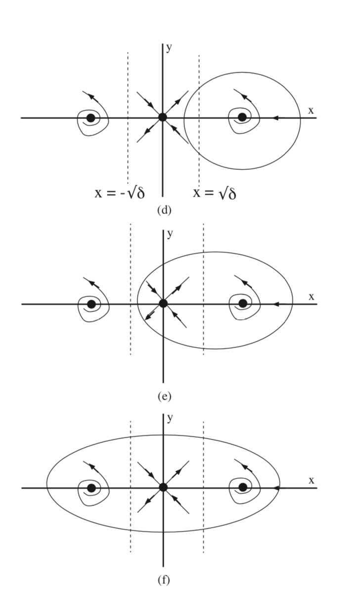
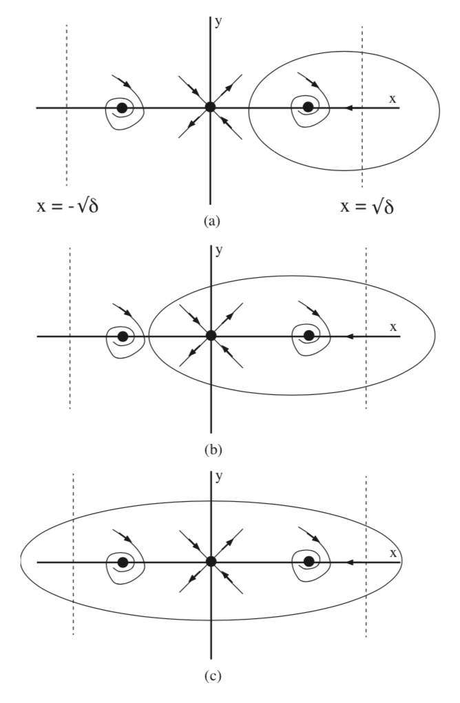
Now we will use Bendixson’s criterion and the index theorem to determine regions in the phase plane where periodic orbits may exist. For this example (7.22) is given by:

\[-\delta+x^2. \label{7.33}\]

Hence the two vertical lines \(x = -\sqrt{\delta}\) and \(x = \sqrt{\delta}\) divide the phase plane into three regions where periodic orbits cannot exist entirely in one of these regions (or else Bendixson’s criterion would be violated). There are two cases to be considered for the location of these vertical lines with respect to the equilibria: \(\delta > 1\) and \(0 < \delta < 1\).

In Fig. 7.1 we show three possibilities (they do not exhaust all possible cases) for the existence of periodic orbits that would satisfy Bendixson’s criterion in the case \(\delta > 1\). However, (b) is not possible because it violates the index theorem.

Figure 7.1: The case \(\delta > 1\). Possibilities for periodic orbits that satisfy Bendixson’s criterion. However, (b) is not possible because it violates the index theorem.

In Fig. 7.2 we show three possibilities (they do not exhaust all possible cases) for the existence of periodic orbits that would satisfy Bendixson’s criterion in the case \(0 < \delta < 1\). However, (e) is not possible because it violates the index theorem.

Figure 7.2: The case \(0 < \delta < 1\). Possibilities for periodic orbits that satisfy Bendixson’s criterion. However, (e) is not possible because it violates the index theorem.