
8.1: Bifurcation of Equilibria I
- Page ID
- 24179

We will now study the topic of bifurcation of equilibria of autonomous vector fields, or ‘’what happens as an equilibrium point loses hyperbolicity as a parameter is varied?” We will study this question through a series of examples, and then consider what the examples teach us about the ‘’general situation” (and what this might be).
ExAMPLE \(\PageIndex{22}\): The Saddle-Node Bifurcation
Consider the following nonlinear, autonomous vector field on \(\mathbb{R}^2\):
\(\dot{x} = \mu x^2\),
\[\dot{y} = y, (x, y) \in \mathbb{R}^2, \label{8.1}\]
where \(\mu\) is a (real) parameter. The equilibrium points of (8.1) are given by:
\[(x, y) = (\sqrt{μ}, 0), (-\sqrt{μ}, 0). \label{8.2}\]
It is easy to see that there are no equilibrium points for \(\mu < 0\), one equilibrium point for \(\mu = 0\), and two equilibrium points for \(\mu > 0\).
The Jacobian of the vector field evaluated at each equilibrium point is given by:
\[(\sqrt{μ}, 0): \begin{pmatrix} {-2\sqrt{μ}}&{0}\\ {0}&{-1} \end{pmatrix}, \label{8.3}\]
from which it follows that the equilibria are hyperbolic and asymptotically stable for \(\mu > 0\), and nonhyperbolic for \(\mu = 0\).
\[(-\sqrt{μ}, 0): \begin{pmatrix} {2\sqrt{μ}}&{0}\\ {0}&{1} \end{pmatrix} \label{8.4}\]
from which it follows that the equilibria are hyperbolic saddle points for \(\mu > 0\), and nonhyperbolic for \(\mu = 0\). We emphasize again that there are no equilibrium points for \(\mu < 0\).
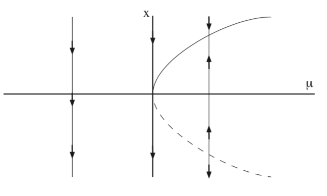
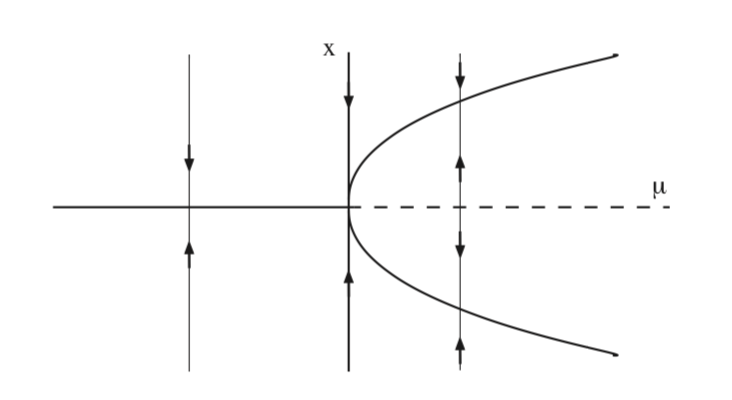
As a result of the "structure" of (8.1) we can easily represent the behavior of the equilibria as a function of \(\mu\) in a bifurcation diagram. That is, since the x and y components of (8.1) are "decoupled", and the change in the number and stability of equilibria us completely captured by the x coordinates, we can plot the x component of the vector field as a function of \(\mu\), as we show in Fig. 8.1.
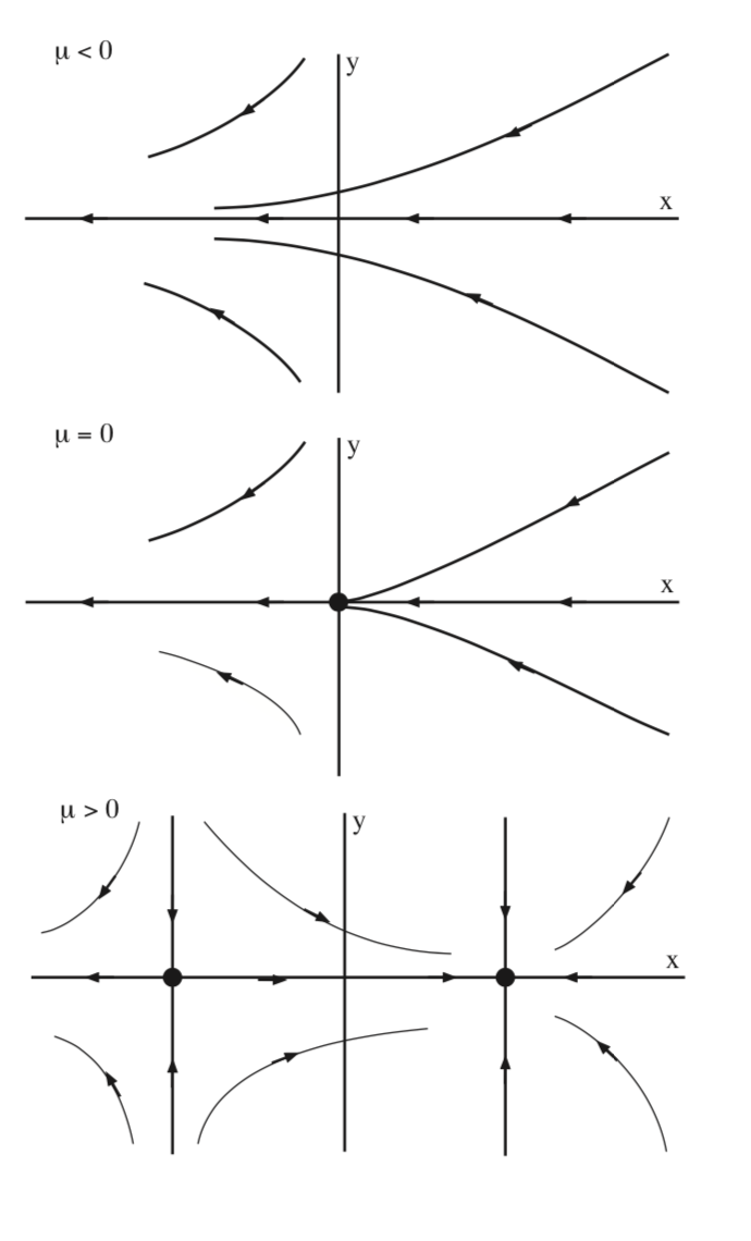
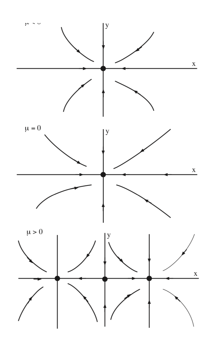
In Fig. 8.2 we illustrate the bifurcation of equilibria for (8.1) in the \(x - y\) plane.
This type of bifurcation is referred to as a saddle-node bifurcation (occasionally it may also be referred to as a fold bifurcation or tangent bifurcation, but these terms are used less frequently).
The key characteristic of the saddle-node bifurcation is the following. As a parameter (\(\mu\)) is varied, the number of equilibria change from zero to two, and the change occurs at a parameter value corresponding to the two equilibria coalescing into one nonhyperbolic equilibrium.
\(\mu\) is called the bifurcation parameter and \(\mu = 0\) is called the bifurcation point.
Example \(\PageIndex{23}\) (The Transcritical Bifurcation)
Consider the following nonlinear, autonomous vector field on \(\mathbb{R}^2\):
\(\dot{x} = \mu x-x^2\),
\[\dot{y} = y, (x, y) \in \mathbb{R}^2, \label{8.5}\]
where \(\mu\) is a (real) parameter. The equilibrium points of (8.5) are given by:
\[(x, y) = (0, 0), (\mu, 0). \label{8.6}\]
The Jacobian of the vector field evaluated at each equilibrium point is given by:
\[(0,0) \begin{pmatrix} {\mu}&{0}\\ {0}&{-1} \end{pmatrix} \label{8.7}\]
\[(\mu, 0) \begin{pmatrix} {-\mu}&{0}\\ {0}&{1} \end{pmatrix} \label{8.8}\]
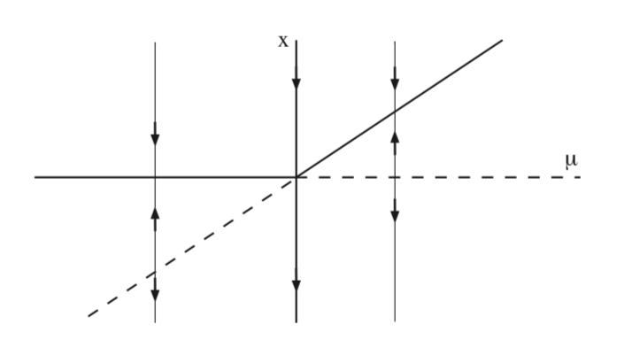
from which it follows that (0, 0) is asymptotically stable for \(\mu < 0\), and a hyperbolic saddle for \(\mu > 0\), and \((\mu, 0)\) is a hyperbolic saddle for \(\mu < 0\) and asymptotically stable for \(\mu > 0\). These two lines of fixed points cross at \(\mu = 0\), at which there is only one, nonhyperbolic fixed point.
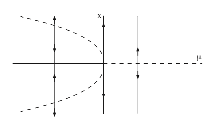
In Fig. 8.3 we show the bifurcation diagram for (8.5) in the \(\mu - x\) plane.
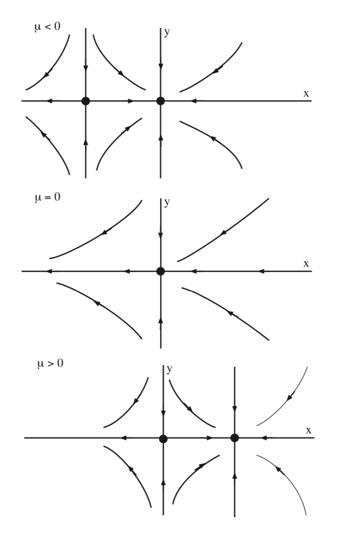
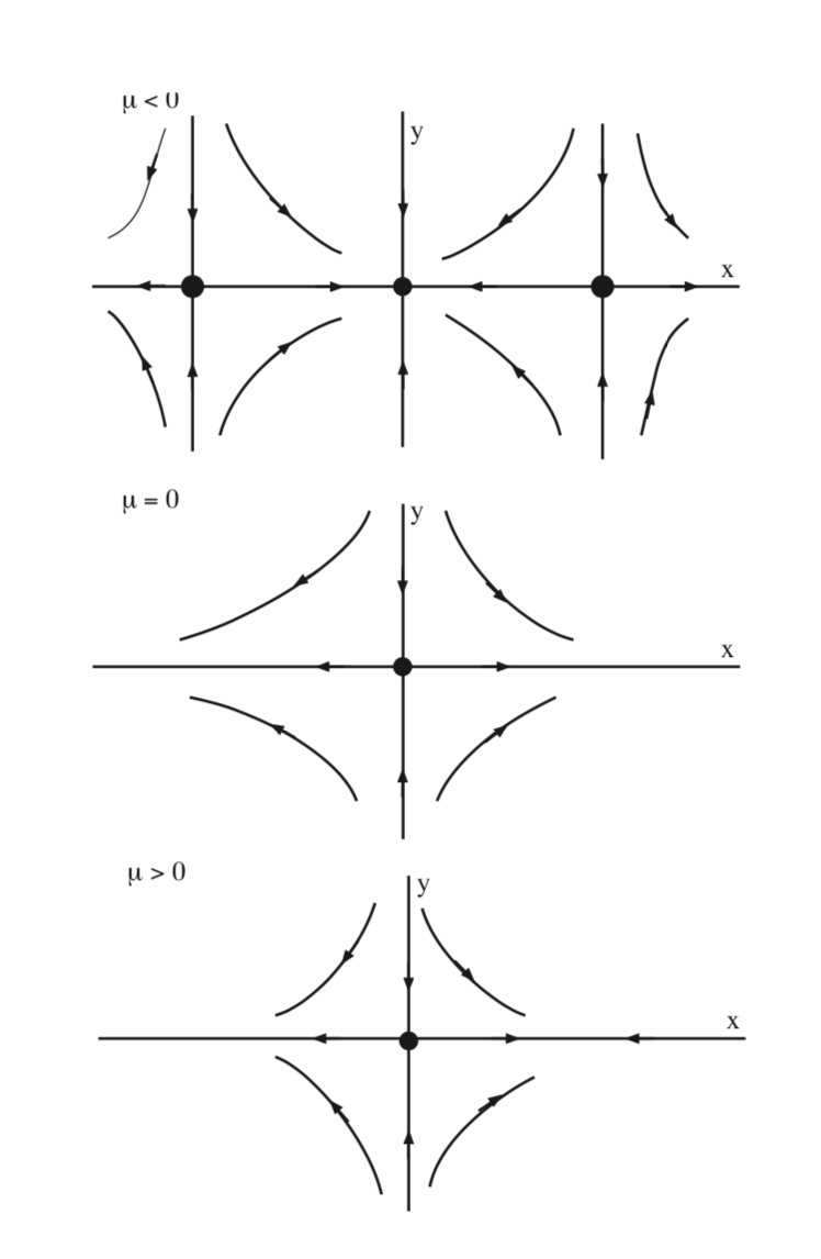
In Fig. 8.4 we illustrate the bifurcation of equilibria for (8.5) in the \(x - y\) plane for \(\mu < 0\), \(\mu = 0\), and \(\mu > 0\).
This type of bifurcation is referred to as a transcritical bifurcation.
The key characteristic of the transcritical bifurcation is the following. As a parameter (\(\mu\)) is varied, the number of equilibria change from two to one, and back to two, and the change in number of equilibria occurs at a parameter value corresponding to the two equilibria coalescing into one nonhyperbolic equilibrium.
ExAMPLE \(\PageIndex{24}\) (The (Supercritical) Pitchfork Bifurcation).
Consider the following nonlinear, autonomous vector field on \(\mathbb{R}^2\):
\(\dot{x} = \mu x-x^3\),
\[\dot{y} = -y, (x, y) \in \mathbb{R}^2, \label{8.9}\]
where \(\mu\) is a (real) parameter. The equilibrium points of (8.9) are given by:
\[(x, y) = (0, 0), (\sqrt{\mu}, 0), (-\sqrt{\mu}, 0) \label{8.10}\]
The Jacobian of the vector field evaluated at each equilibrium point is given by:
\[(0, 0) \begin{pmatrix} {\mu}&{0}\\ {0}&{1} \end{pmatrix} \label{8.11}\]
\[(\pm \sqrt{μ}, 0) \begin{pmatrix} {-2\mu}&{0}\\ {0}&{1} \end{pmatrix} \label{8.12}\]
from which it follows that (0, 0) is asymptotically stable for \(\mu < 0\), and a hyperbolic saddle for \(\mu > 0\), and \(( \pm \sqrt{μ}, 0)\) are asymptotically stable for \(\mu > 0\), and do not exist for \(\mu < 0\). These two curves of fixed points pass through zero at \(\mu = 0\), at which there is only one, nonhyperbolic fixed point.
In Fig. 8.5 we show the bifurcation diagram for (8.9) in the \(\mu - x\) plane.
In Fig. 8.6 we illustrate the bifurcation of equilibria for (8.9) in the \(x - y\) plane for \(\mu < 0\), \(\mu = 0\), and \(\mu > 0\).
Example \(\PageIndex{25}\) (The (Subcritical) Pitchfork Bifurcation)
Consider the following nonlinear, autonomous vector field on \(\mathbb{R}^2\):
\(\dot{x} = \mu x+x^3\),
\[\dot{y} = y, (x, y) \in \mathbb{R}^2, \label{8.13}\]
where \(\mu\) is a (real) parameter. The equilibrium points of (8.9) are given by:
\[(x, y) = (0, 0), (\sqrt{μ}, 0), (-\sqrt{μ}, 0). \label{8.14}\]
The Jacobian of the vector field evaluated at each equilibrium point is given by:
\[(0, 0) \begin{pmatrix} {\mu}&{0}\\ {0}&{-1} \end{pmatrix} \label{8.15}\]
\[(\pm \sqrt{\mu}, 0) \begin{pmatrix} {-2\mu}&{0}\\ {0}&{1} \end{pmatrix} \label{8.16}\]
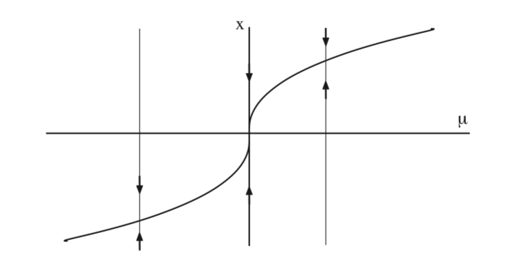
from which it follows that (0, 0) is asymptotically stable for \(\mu < 0\), and a hyperbolic saddle for \(\mu > 0\), and \((\pm \sqrt{μ}, 0)\) are hyperbolic saddles for \(\mu < 0\), and do not exist for \(\mu > 0\). These two curves of fixed points pass through zero at \(\mu = 0\), at which there is only one, nonhyperbolic fixed point. In Fig. 8.7 we show the bifurcation diagram for (8.13) in the \(\mu - x\) plane.
In Fig. 8.8 we illustrate the bifurcation of equilibria for (8.9) in the \(x - y\) plane for \(\mu < 0\), \(\mu = 0\), and \(\mu > 0\).
We note that the phrase supercritical pitchfork bifurcation is also referred to as a soft loss of stability and the phrase subcritical pitchfork bifurcation is referred to as a hard loss of stability. What this means is the following. In the supercritical pitchfork bifurcation as \(\mu\) goes from negative to positive the equilibrium point loses stability, but as \(\mu\) increases past zero the trajectories near the origin are bounded in how far away from the origin they can move. In the subcritical pitchfork bifurcation the origin loses stability as \(\mu\) increases from negative to positive, but trajectories near the unstable equilibrium can become unbounded.
It is natural to ask the question,
"what is common about these three examples of bifurcations of fixed points of one dimensional autonomous vector fields?" We note the following.
- A necessary (but not sufficient) for bifurcation of a fixed point is nonhyperbolicity of the fixed point.
- The "nature" of the bifurcation (e.g. numbers and stability of fixed points that are created or destroyed) is determined by the form of the nonlinearity.
But we could go further and ask what is in common about these examples that could lead to a definition of the bifurcation of a fixed point for autonomous vector fields? From the common features we give the following definition.
Definition 21 (Bifurcation of a fixed point of a one dimensional autonomous vector field)
We consider a one dimensional autonomous vector field depending on a parameter, \(\mu\). We assume that at a certain parameter value it has a fixed point that is not hyperbolic. We say that a bifurcation occurs at that "nonhyperbolic parameter value" if for \(\mu\) in a neighborhood of that parameter value the number of fixed points and their stability changes.
Finally, we finish the discussion of bifurcations of a fixed point of one dimensional autonomous vector fields with an example showing that a nonhyperbolic fixed point may not bifurcate as a parameter is varied, i.e. non-hyperbolicity is a necessary, but not sufficient, condition for bifurcation.
Example \(\PageIndex{26}\)
We consider the one dimensional autonomous vector field:
\[\dot{x} =\mu-x^3, x \in \mathbb{R}, \label{8.17}\]
where \(\mu\) is a parameter. This vector field has a nonhyperbolic fixed point at x = 0 for \(\mu = 0\). The curve of fixed points in the \(\mu - x\) plane is given by \(\mu = x^3\), and the Jacobian of the vector field is \(-3x^2\), which is strictly negative at all fixed points, except the nonhyperbolic fixed point at the origin.
In fig. 8.9 we plot the fixed points as a function of \(\mu\).
We see that there is no change in the number or stability of the fixed points for \(\mu > 0\) and \(\mu < 0\). Hence, no bifurcation.