1.3: Partial Differential Equations

The same procedure as above applied to the following multiple integral leads to a second-order quasilinear partial differential equation. Set

$$E(v)=\int_\Omega\ F(x,v,\nabla v)\ dx,\]

where $\Omega\subset\mathbb{R}^n$ is a domain, $x=(x_1,\ldots,x_n)$, $v=v(x):\ \Omega\mapsto\mathbb{R}^1$, and $\nabla v=(v_{x_1},\ldots,v_{x_n})$. Assume that the function $F$ is sufficiently regular in its arguments. For a given function $h$, defined on $\partial\Omega$, set

$$V=\{v\in C^2(\overline{\Omega}):\ v=h\ \mbox{on}\ \partial\Omega\}.\]

Euler equation. Let $u\in V$ be a solution of (P), then

$$\sum_{i=1}^n\frac{\partial}{\partial x_i}F_{u_{x_i}}-F_u=0$$

in $\Omega$.

Proof. Exercise. Hint: Extend the above fundamental lemma of the calculus of variations to the case of multiple integrals. The interval $(x_0-\delta,x_0+\delta)$ in the definition of $\phi$ must be replaced by a ball with center at $x_0$ and radius $\delta$.

Example 1.2.2.1: Dirichlet integral

In two dimensions the Dirichlet integral is given by

$$D(v)=\int_\Omega\ \left(v_x^2+v_y^2\right)\ dxdy\]

and the associated Euler equation is the Laplace equation $\triangle u=0$ in $\Omega$.

Thus, there is natural relationship between the boundary value problem

$$\triangle u=0\ \ \mbox{in}\ \Omega,\ u=h\ \ \mbox{on}\ \ \partial\Omega\]

and the variational problem

$$\min_{v\in V}\ D(v).\]

But these problems are not equivalent in general. It can happen that the boundary value problem has a solution but the variational problem has no solution, for an example see Courant and Hilbert [4], Vol. 1, p. 155, where $h$ is a continuous function and the associated solution $u$ of the boundary value problem has no finite Dirichlet integral.

The problems are equivalent, provided the given boundary value function $h$ is in the class
$H^{1/2}(\partial\Omega)$, see Lions and Magenes [14].

Example 1.2.2.2: Minimal surface equation

The non-parametric minimal surface problem in two dimensions is to find a minimizer $u=u(x_1,x_2)$ of the problem

$$\min_{v\in V}\int_\Omega\ \sqrt{1+v_{x_1}^2+v_{x_2}^2}\ dx,\]

where for a given function $h$ defined on the boundary of the domain $\Omega$

$$V=\{v\in C^1(\overline{\Omega}):\ v=h\ \mbox{on}\ \partial\Omega\}.\]

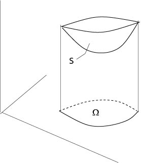
Figure 1.2.2.1: Comparison surface

Suppose that the minimizer satisfies the regularity assumption $u\in C^2(\Omega)$, then
$u$ is a solution of the minimal surface equation (Euler equation) in $\Omega$

$$\begin{equation} \label{mse} \frac{\partial}{\partial x_1}\left(\frac{u_{x_1}}{\sqrt{1+|\nabla u|^2}}\right)+ \frac{\partial}{\partial x_2}\left(\frac{u_{x_2}}{\sqrt{1+|\nabla u|^2}}\right)=0. \end{equation}$$

In fact, the additional assumption $u\in C^2(\Omega)$ is superfluous since it follows from regularity considerations for quasilinear elliptic equations of second order, see for example Gilbarg and Trudinger [9].

Let $\Omega=\mathbb{R}^2$. Each linear function is a solution of the minimal surface equation ($\ref{mse}$). It was shown by Bernstein [2] that there are no other solutions of the minimal surface quation. This is true also for higher dimensions $n\le7$, see Simons [19].

If $n\ge8$, then there exists also other solutions which define cones, see Bombieri, De Giorgi and Giusti [3].

The linearized minimal surface equation over $u\equiv0$ is the Laplace equation $\triangle u=0$. In $\mathbb{R}^2$ linear functions are solutions but also many other functions in contrast to the minimal surface equation. This striking difference is caused by the strong nonlinearity of the minimal surface equation.

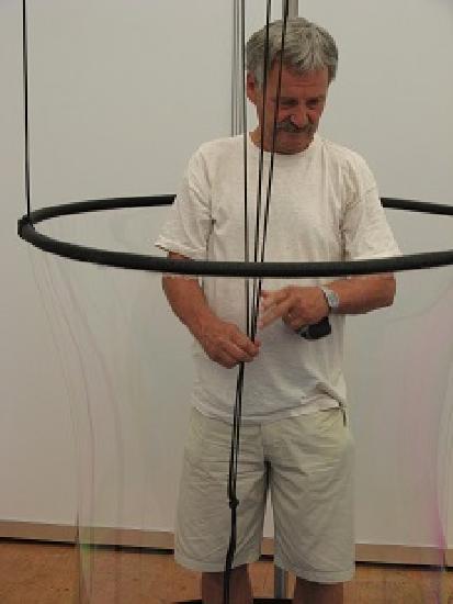
More general minimal surfaces are described by using parametric representations. An example is shown in Figure 1.2.2.2¹. See [18], pp. 62, for example, for rotationally symmetric minimal surfaces.

Figure 1.2.2.2: Rotationally symmetric minimal surface

¹An experiment from Beutelspacher's Mathetikum, Wissenschaftsjahr 2008, Leipzig

Neumann type boundary value problems

Set $V=C^1(\overline{\Omega})$ and

$$E(v)=\int_\Omega\ F(x,v,\nabla v)\ dx-\int_{\partial\Omega}\ g(x,v)\ ds,\]

where $F$ and $g$ are given sufficiently regular functions and $\Omega\subset\mathbb{R}^n$ is a bounded and sufficiently regular domain.
Assume $u$ is a minimizer of $E(v)$ in $V$, that is

$$u\in V:\ \ E(u)\le E(v)\ \ \mbox{for all}\ v\in V,\]

then

$$\begin{eqnarray*} \int_\Omega\ \big(\sum_{i=1}^nF_{u_{x_i}}(x,u,\nabla u)\phi_{x_i}&+& F_u(x,u,\nabla u)\phi\big)\ dx\\ &-& \int_{\partial\Omega}\ g_u(x,u)\phi\ ds =0 \end{eqnarray*}$$
for all $\phi\in C^1(\overline{\Omega})$. Assume additionally $u\in C^2(\Omega)$, then $u$ is a solution of the Neumann type boundary value problem
$$\begin{eqnarray*} \sum_{i=1}^n\frac{\partial}{\partial x_i}F_{u_{x_i}}-F_u&=&0\ \ \mbox{in}\ \Omega\\ \sum_{i=1}^nF_{u_{x_i}}\nu_i-g_u&=&0\ \ \mbox{on}\ \partial\Omega, \end{eqnarray*}$$

where $\nu=(\nu_1,\ldots,\nu_n)$ is the exterior unit normal at the boundary $\partial\Omega$. This follows after integration by parts from the basic lemma of the calculus of variations.

Example 1.2.2.3: Laplace equation

Set

$$E(v)=\frac{1}{2}\int_\Omega\ |\nabla v|^2\ dx-\int_{\partial\Omega}\ h(x)v\ ds,\]

then the associated boundary value problem is

$$\begin{eqnarray*} {\triangle} u&=&0\ \ \mbox{in}\ \Omega\\ \frac{\partial u}{\partial\nu}&=&h\ \ \mbox{on}\ \partial\Omega. \end{eqnarray*}$$

Example 1.2.2.4: Capillary equation

Let $\Omega\subset\mathbb{R}^2$ and set

$$E(v)=\int_\Omega\ \sqrt{1+|\nabla v|^2}\ dx+\frac{\kappa}{2}\int_\Omega\ v^2\ dx -\cos\gamma\int_{\partial\Omega}\ v\ ds.\]

Here $\kappa$ is a positive constant (capillarity constant) and $\gamma$ is the (constant) boundary contact angle, i. e., the angle between the container wall and the capillary surface, defined by $v=v(x_1,x_2)$, at the boundary.

Then the related boundary value problem is

$$\begin{eqnarray*} \text{div}\ (Tu)&=&\kappa u\ \ \mbox{in}\ \Omega\\ \nu\cdot Tu&=&\cos\gamma \ \mbox{on}\ \partial\Omega, \end{eqnarray*}$$
where we use the abbreviation

$$Tu=\frac{\nabla u}{\sqrt{1+|\nabla u|^2}},\]

div $(Tu)$ is the left hand side of the minimal surface equation ($\ref{mse}$) and it is twice the mean curvature of the surface defined by $z=u(x_1,x_2)$, see an exercise.

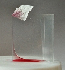
The above problem describes the ascent of a liquid, water for example, in a vertical cylinder with cross section $\Omega$. Assume the gravity is directed downwards in the direction of the negative $x_3$-axis. Figure 1.2.2.3 shows that liquid can rise along a vertical wedge which is a consequence of the strong non-linearity of the underlying equations, see Finn [7]. This photo was taken from [15].

Figure 1.2.2.3: Ascent of liquid in a wedge

Contributors and Attributions

• Prof. Dr. Erich Miersemann (Universität Leipzig)

• Integrated by Justin Marshall.