Mathematics LibreTexts

3.4: More Realistic Examples of Boundary and Initial Conditions

  • Page ID
    8358
  • \( \newcommand{\vecs}[1]{\overset { \scriptstyle \rightharpoonup} {\mathbf{#1}} } \)

    \( \newcommand{\vecd}[1]{\overset{-\!-\!\rightharpoonup}{\vphantom{a}\smash {#1}}} \)

    \( \newcommand{\id}{\mathrm{id}}\) \( \newcommand{\Span}{\mathrm{span}}\)

    ( \newcommand{\kernel}{\mathrm{null}\,}\) \( \newcommand{\range}{\mathrm{range}\,}\)

    \( \newcommand{\RealPart}{\mathrm{Re}}\) \( \newcommand{\ImaginaryPart}{\mathrm{Im}}\)

    \( \newcommand{\Argument}{\mathrm{Arg}}\) \( \newcommand{\norm}[1]{\| #1 \|}\)

    \( \newcommand{\inner}[2]{\langle #1, #2 \rangle}\)

    \( \newcommand{\Span}{\mathrm{span}}\)

    \( \newcommand{\id}{\mathrm{id}}\)

    \( \newcommand{\Span}{\mathrm{span}}\)

    \( \newcommand{\kernel}{\mathrm{null}\,}\)

    \( \newcommand{\range}{\mathrm{range}\,}\)

    \( \newcommand{\RealPart}{\mathrm{Re}}\)

    \( \newcommand{\ImaginaryPart}{\mathrm{Im}}\)

    \( \newcommand{\Argument}{\mathrm{Arg}}\)

    \( \newcommand{\norm}[1]{\| #1 \|}\)

    \( \newcommand{\inner}[2]{\langle #1, #2 \rangle}\)

    \( \newcommand{\Span}{\mathrm{span}}\) \( \newcommand{\AA}{\unicode[.8,0]{x212B}}\)

    \( \newcommand{\vectorA}[1]{\vec{#1}}      % arrow\)

    \( \newcommand{\vectorAt}[1]{\vec{\text{#1}}}      % arrow\)

    \( \newcommand{\vectorB}[1]{\overset { \scriptstyle \rightharpoonup} {\mathbf{#1}} } \)

    \( \newcommand{\vectorC}[1]{\textbf{#1}} \)

    \( \newcommand{\vectorD}[1]{\overrightarrow{#1}} \)

    \( \newcommand{\vectorDt}[1]{\overrightarrow{\text{#1}}} \)

    \( \newcommand{\vectE}[1]{\overset{-\!-\!\rightharpoonup}{\vphantom{a}\smash{\mathbf {#1}}}} \)

    \( \newcommand{\vecs}[1]{\overset { \scriptstyle \rightharpoonup} {\mathbf{#1}} } \)

    \( \newcommand{\vecd}[1]{\overset{-\!-\!\rightharpoonup}{\vphantom{a}\smash {#1}}} \)

    \(\newcommand{\avec}{\mathbf a}\) \(\newcommand{\bvec}{\mathbf b}\) \(\newcommand{\cvec}{\mathbf c}\) \(\newcommand{\dvec}{\mathbf d}\) \(\newcommand{\dtil}{\widetilde{\mathbf d}}\) \(\newcommand{\evec}{\mathbf e}\) \(\newcommand{\fvec}{\mathbf f}\) \(\newcommand{\nvec}{\mathbf n}\) \(\newcommand{\pvec}{\mathbf p}\) \(\newcommand{\qvec}{\mathbf q}\) \(\newcommand{\svec}{\mathbf s}\) \(\newcommand{\tvec}{\mathbf t}\) \(\newcommand{\uvec}{\mathbf u}\) \(\newcommand{\vvec}{\mathbf v}\) \(\newcommand{\wvec}{\mathbf w}\) \(\newcommand{\xvec}{\mathbf x}\) \(\newcommand{\yvec}{\mathbf y}\) \(\newcommand{\zvec}{\mathbf z}\) \(\newcommand{\rvec}{\mathbf r}\) \(\newcommand{\mvec}{\mathbf m}\) \(\newcommand{\zerovec}{\mathbf 0}\) \(\newcommand{\onevec}{\mathbf 1}\) \(\newcommand{\real}{\mathbb R}\) \(\newcommand{\twovec}[2]{\left[\begin{array}{r}#1 \\ #2 \end{array}\right]}\) \(\newcommand{\ctwovec}[2]{\left[\begin{array}{c}#1 \\ #2 \end{array}\right]}\) \(\newcommand{\threevec}[3]{\left[\begin{array}{r}#1 \\ #2 \\ #3 \end{array}\right]}\) \(\newcommand{\cthreevec}[3]{\left[\begin{array}{c}#1 \\ #2 \\ #3 \end{array}\right]}\) \(\newcommand{\fourvec}[4]{\left[\begin{array}{r}#1 \\ #2 \\ #3 \\ #4 \end{array}\right]}\) \(\newcommand{\cfourvec}[4]{\left[\begin{array}{c}#1 \\ #2 \\ #3 \\ #4 \end{array}\right]}\) \(\newcommand{\fivevec}[5]{\left[\begin{array}{r}#1 \\ #2 \\ #3 \\ #4 \\ #5 \\ \end{array}\right]}\) \(\newcommand{\cfivevec}[5]{\left[\begin{array}{c}#1 \\ #2 \\ #3 \\ #4 \\ #5 \\ \end{array}\right]}\) \(\newcommand{\mattwo}[4]{\left[\begin{array}{rr}#1 \amp #2 \\ #3 \amp #4 \\ \end{array}\right]}\) \(\newcommand{\laspan}[1]{\text{Span}\{#1\}}\) \(\newcommand{\bcal}{\cal B}\) \(\newcommand{\ccal}{\cal C}\) \(\newcommand{\scal}{\cal S}\) \(\newcommand{\wcal}{\cal W}\) \(\newcommand{\ecal}{\cal E}\) \(\newcommand{\coords}[2]{\left\{#1\right\}_{#2}}\) \(\newcommand{\gray}[1]{\color{gray}{#1}}\) \(\newcommand{\lgray}[1]{\color{lightgray}{#1}}\) \(\newcommand{\rank}{\operatorname{rank}}\) \(\newcommand{\row}{\text{Row}}\) \(\newcommand{\col}{\text{Col}}\) \(\renewcommand{\row}{\text{Row}}\) \(\newcommand{\nul}{\text{Nul}}\) \(\newcommand{\var}{\text{Var}}\) \(\newcommand{\corr}{\text{corr}}\) \(\newcommand{\len}[1]{\left|#1\right|}\) \(\newcommand{\bbar}{\overline{\bvec}}\) \(\newcommand{\bhat}{\widehat{\bvec}}\) \(\newcommand{\bperp}{\bvec^\perp}\) \(\newcommand{\xhat}{\widehat{\xvec}}\) \(\newcommand{\vhat}{\widehat{\vvec}}\) \(\newcommand{\uhat}{\widehat{\uvec}}\) \(\newcommand{\what}{\widehat{\wvec}}\) \(\newcommand{\Sighat}{\widehat{\Sigma}}\) \(\newcommand{\lt}{<}\) \(\newcommand{\gt}{>}\) \(\newcommand{\amp}{&}\) \(\definecolor{fillinmathshade}{gray}{0.9}\)

    A String with Fixed Endpoints

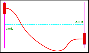
    Consider a string fixed at \(x=0\) and \(x=a\), as in Figure \(\PageIndex{1}\)

    string1.png
    Figure \(\PageIndex{1}\): A string with fixed endpoints.

    It satisfies the wave equation

    \[\frac{1}{c^2} \frac{\partial^2 u}{\partial t^2} = \frac{\partial^2 u}{\partial x^2},\space \space\space\qquad 0<x<a, \nonumber \]

    with boundary conditions \[u(0,t) = u(a,t) = 0, \qquad t>0, \nonumber \]

    and initial conditions,

    \[u(x,0) = f(x), \frac{\partial u}{\partial x}(x,0) = g(x). \nonumber \]

    A String with Freely Floating Endpoints

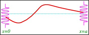
    Consider a string with ends fastened to air bearings that are fixed to a rod orthogonal to the \(x\)-axis. Since the bearings float freely there should be no force along the rods, which means that the string is horizontal at the bearings (Figure \(\PageIndex{2}\)).
    string2.png
    Figure \(\PageIndex{2}\): A string with floating endpoints.

    It satisfies the wave equation with the same initial conditions as above, but the boundary conditions now are \[\frac{\partial u}{\partial x} (0,t) = \frac{\partial u}{\partial x} (a,t) = 0, \space\space \qquad t>0. \nonumber \] These are clearly of von Neumann type.

    A String with Endpoints Fixed to Strings

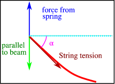
    To illustrate mixed boundary conditions we make an even more complicated contraption where we fix the endpoints of the string to springs, with equilibrium at \(y=0\), see Figure \(\PageIndex{3}\) for a sketch.
    string3.png
    Figure \(\PageIndex{3}\): A string with endpoints fixed to springs.

    Hook’s law states that the force exerted by the spring (along the \(y\) axis) is \(F=-ku(0,t)\), where \(k\) is the spring constant. This must be balanced by the force the string on the spring, which is equal to the tension \(T\) in the string. The component parallel to the \(y\) axis is \(T\sin\alpha\), where \(\alpha\) is the angle with the horizontal, see Figure \(\PageIndex{4}\).
    string3b.png
    Figure \(\PageIndex{4}\): the balance of forces at one endpoint of the string of Figure \(\PageIndex{3}\)

    For small \(\alpha\) we have

    \[\sin\alpha \approx \tan\alpha = \frac{\partial u}{\partial x}(0,t). \nonumber \]

    Since both forces should cancel we find

    \[ {u}(0,t) -\frac{T}{k} \frac{\partial u}{\partial x}(0,t) = 0, \qquad t>0, \nonumber \]

    and

    \[ u(a,t) -\frac{T}{k} \frac{\partial u}{\partial x}(a,t) = 0, \nonumber \]

    These are mixed boundary conditions.


    This page titled 3.4: More Realistic Examples of Boundary and Initial Conditions is shared under a CC BY-NC-SA 2.0 license and was authored, remixed, and/or curated by Niels Walet via source content that was edited to the style and standards of the LibreTexts platform.

    • Was this article helpful?