2.3: The General Planar Truss

Last updated
Save as PDF

Page ID: 21807

$ \newcommand{\vecs}[1]{\overset { \scriptstyle \rightharpoonup} {\mathbf{#1}} } $ $ \newcommand{\vecd}[1]{\overset{-\!-\!\rightharpoonup}{\vphantom{a}\smash {#1}}} $$\newcommand{\id}{\mathrm{id}}$ $ \newcommand{\Span}{\mathrm{span}}$ $ \newcommand{\kernel}{\mathrm{null}\,}$ $ \newcommand{\range}{\mathrm{range}\,}$ $ \newcommand{\RealPart}{\mathrm{Re}}$ $ \newcommand{\ImaginaryPart}{\mathrm{Im}}$ $ \newcommand{\Argument}{\mathrm{Arg}}$ $ \newcommand{\norm}[1]{\| #1 \|}$ $ \newcommand{\inner}[2]{\langle #1, #2 \rangle}$ $ \newcommand{\Span}{\mathrm{span}}$ $\newcommand{\id}{\mathrm{id}}$ $ \newcommand{\Span}{\mathrm{span}}$ $ \newcommand{\kernel}{\mathrm{null}\,}$ $ \newcommand{\range}{\mathrm{range}\,}$ $ \newcommand{\RealPart}{\mathrm{Re}}$ $ \newcommand{\ImaginaryPart}{\mathrm{Im}}$ $ \newcommand{\Argument}{\mathrm{Arg}}$ $ \newcommand{\norm}[1]{\| #1 \|}$ $ \newcommand{\inner}[2]{\langle #1, #2 \rangle}$ $ \newcommand{\Span}{\mathrm{span}}$$\newcommand{\AA}{\unicode[.8,0]{x212B}}$

Let us now consider something that resembles the mechanical prospection problem introduced in the introduction to matrix methods to matrix methods for mechanical systems. In the figure below we offer a crude mechanical model of a planar tissue, say, e.g., an excised sample of the wall of a vein.

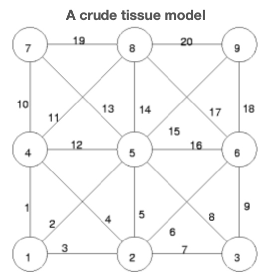
Screen Shot 2020-08-23 at 9.50.06 PM.png — Figure 1.

Elastic fibers, numbered 1 through 20, meet at nodes, numbered 1 through 9. We limit our observation to the motion of the nodes by denoting the horizontal and vertical displacements of node j by $x_{2j-1}$ (horizontal) and $x_{2j}$ (vertical), respectively. Retaining the convention that down and right are positive we note that the elongation of fiber 1 is

\[e_{1} = x_{2}-x_{8} \nonumber\]

while that of fiber 3 is

\[e_{3} = x_{3}-x_{1} \nonumber\].

As fibers 2 and 4 are neither vertical nor horizontal their elongations, in terms of nodal displacements, are not so easy to read off. This is more a nuisance than an obstacle however, for noting our discussion of elongation in the small planar truss module, the elongation is approximately just the stretch along its undeformed axis. With respect to fiber 2, as it makes the angle $-\frac{\pi}{4}$ with respect to the positive horizontal axis, we find

\[e_{2} = x_{9} \cos(-\frac{\pi}{4})-x_{10} \sin(-\frac{\pi}{4}) = \frac{x_{9}-x_{1}+x_{2}-x_{10}}{\sqrt{22}} \nonumber\]

Similarly, as fiber 4 makes the angle $-\frac{3 \pi}{4}$ with respect to the positive horizontal axis, its elongation is

\[e_{4} = x_{7} \cos(-\frac{3\pi}{4})-x_{8} \sin(-\frac{3\pi}{4}) = \frac{x_{3}-x_{7}+x_{4}-x_{8}}{\sqrt{22}} \nonumber\]

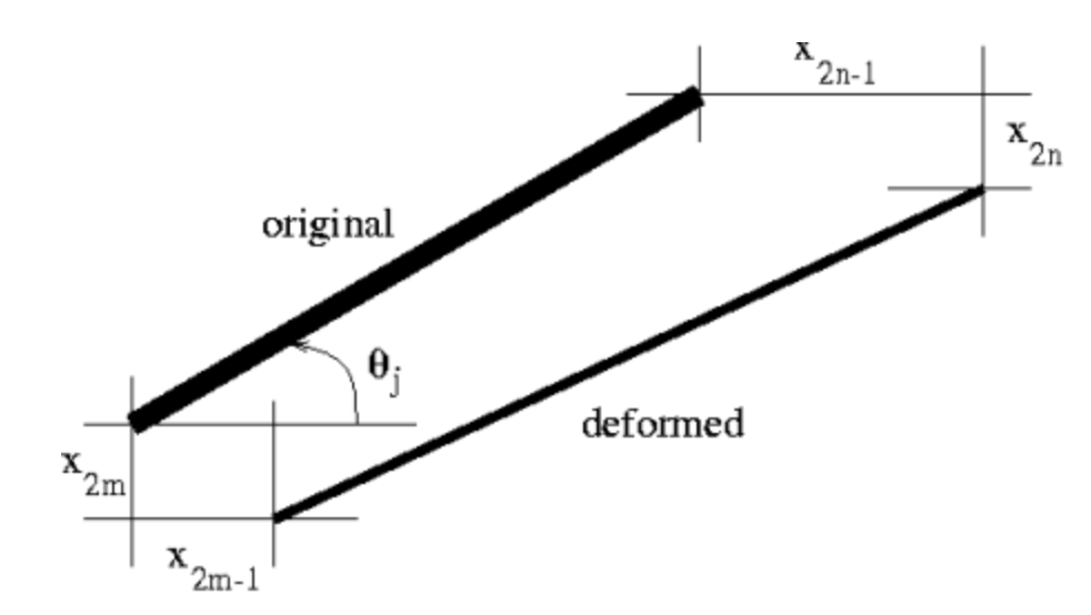
These are both direct applications of the general formula

\[e_{j} = x_{2n-1} \cos(\theta_{j})-x_{2n} \sin(\theta_{j}) \nonumber\]

for fiber j Figure below, connecting node mm to node nn and making the angle $\theta_{j}$ with the positive horizontal axis when node $m$ is assumed to lie at the point $(0, 0)$. The reader should check that our expressions for $e_{1}$ and $e_{3}$ indeed conform to this general formula and that $e_{2}$ and $e_{4}$ agree with ones intuition. For example, visual inspection of the specimen suggests that fiber 2 can not be supposed to stretch (i.e., have positive $e_{2}$) unless $x_{9} > x_{1}$ and/or $x_{2} > x_{10}$. Does this jive with Equation?

Screen Shot 2020-08-23 at 9.59.04 PM.png — Figure 2. Elongation of a generic bar, see Equation.

Applying Equation to each of the remaining fibers we arrive at $\textbf{e} = A\textbf{⁢x}$ where $A$ is 20-by-18, one row for each fiber, and one column for each degree of freedom. For systems of such size with such a well defined structure one naturally hopes to automate the construction. We have done just that in the accompanying M-file and diary. The M-file begins with a matrix of raw data that anyone with a protractor could have keyed in directly from Figure 1.:

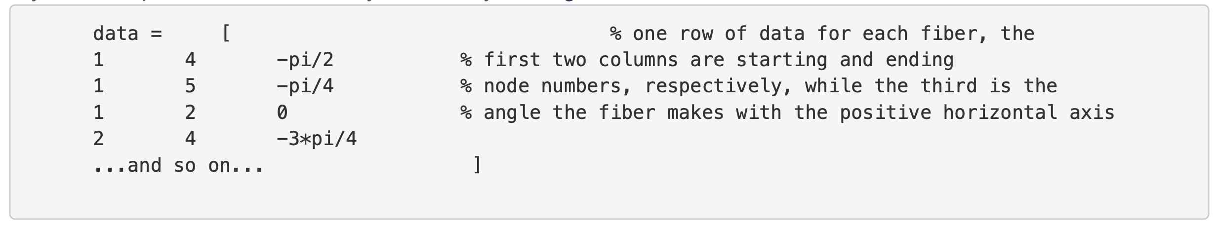
$Screen Shot 2020-08-23 at 10.01.52 PM.png$

This data is precisely what Euqation requires in order to know which columns of $A$ receive the proper $\cos$ or $\sin$. The final $A$ matrix is displayed in the diary.

The next two steps are now familiar. If $K$ denotes the diagonal matrix of fiber stiffnesses and $\textbf{f}$ denotes the vector of nodal forces then

\[\begin{array} {ccc} {\textbf{y} = K \textbf{e}}&{and}&{A^{T} \textbf{y} = \textbf{f}} \nonumber \end{array}\]

and so one must solve $S \textbf{⁢x} = \textbf{f}$ where $S = A^{T}KA$. In this case there is an entire three--dimensional class of $\textbf{z}$ for which $A \textbf{⁢z} = \textbf{0}$ and therefore $S \textbf{⁢z} = \textbf{0}$ e.g., two translations and a rotation. As a result $S$ is singular and x = S\f in MATLAB will get us nowhere. The way out is to recognize that $S$ has $18-3 = 15$ stable modes and that if we restrict $S$ to 'act' only in these directions then it 'should' be invertible. We will begin to make these notions precise in discussions on the Fundamental Theorem of Linear Algebra. For now let us note that every matrix possesses such a pseudo-inverse and that it may be computed in MATLAB via the pinv command. Supposing the fiber stiffnesses to each be one and the edge traction to be of the form

\[\textbf{f} =\begin{pmatrix} {-1}&{1}&{0}&{1}&{1}&{1}&{-1}&{0}&{0}&{0}&{1}&{0}&{-1}&{-1}&{0}&{-1}&{1}&{-1} \end{pmatrix}^T \nonumber\],

we arrive at $\textbf{x}$ via x=pinv(S)*f and offer below its graphical representation.

Before-After Plot