2.2: A Small Planar Truss

We return once again to the biaxial testing problem, introduced in the uniaxial truss module. It turns out that singular matrices are typical in the biaxial testing problem. As our initial step into the world of such planar structures let us consider the simple truss in the figure of a simple swing.

Figure 1.

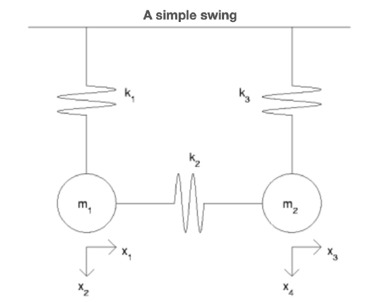
We denote by \(x_{1}\) and \(x_{2}\) the respective horizontal and vertical displacements of \(m_{1}\) (positive is right and down). Similarly, \(f_{1}\) and \(f_{2}\) will denote the associated components of force. The corresponding displacements and forces at \(m_{2}\) will be denoted by \(x_{3}, x_{4}\) and \(f_{3}, f_{4}\) In computing the elongations of the three springs we shall make reference to their unstretched lengths, \(L_{1}, L_{2}\) and \(L_{3}\)

Now, if spring 1 connects \(\{0, -L_{1}\}\) to \(\{0, 1\}\) when at rest and \(\{0, -L_{1}\}\) to \(\{x_{1}, x_{2}\}\) when stretched then its elongation is simply

\[e_{1} = \sqrt{2x_{1}^{2}+(x_{2}+L_{1})^2}-L_{1} \nonumber\]

The price one pays for moving to higher dimensions is that lengths are now expressed in terms of square roots. The upshot is that the elongations are not linear combinations of the end displacements as they were in the uniaxial case. If we presume, however, that the loads and stiffnesses are matched in the sense that the displacements are small compared with the original lengths, then we may effectively ignore the nonlinear contribution in Equation. In order to make this precise we need only recall the Taylor development of the square root of \((1+t)\)

The Taylor development of \(\sqrt{21+t}\) about \(t = 0\) is

\[\sqrt{21+t} = 1+\frac{t}{2}+O(t^2) \nonumber\]

where the latter term signifies the remainder.

With regard to \(e_{1}\) this allows

\[e_{1} = \sqrt{2x_{1}^{2}+x_{2}^{2}+2x_{2}L_{1}+L_{1}^2}-L_{1} \nonumber\]

\[= L_{1} \sqrt{21+\frac{x_{1}^{2}+x_{2}^{2}}{L_{1}^{2}}+\frac{2x_{2}}{L_{1}}}-L_{1} \nonumber\]

\[e_{1} = L_{1}+\frac{x_{1}^{2}+x_{2}^{2}}{2L_{1}^{2}}+x_{2}+L_{1}O((\frac{x_{1}^{2}+x_{2}^{2}}{L_{1}^{2}}+\frac{2x_{2}}{L_{1}})^{2})-L_{1} \nonumber\]

\[= \frac{x_{1}^{2}+x_{2}^{2}}{2L_{1}^{2}}+x_{2}+L_{1}O((\frac{x_{1}^{2}+x_{2}^{2}}{L_{1}^{2}}+\frac{2x_{2}}{L_{1}})^{2}) \nonumber\]

If we now assume that

\(\frac{x_{1}^{2}+x_{2}^{2}}{L_{1}^{2}}\) is small compared with \(x_{2}\)

then, as the O term is even smaller, we may neglect all but the first terms in the above and so arrive at

\[e_{1} = x_{2} \nonumber\]

To take a concrete example, if \(L_{1}\) is one meter and \(x_{1}\) and \(x_{2}\) are each one centimeter, then \(x_{2}\) is one hundred times \(\frac{x_{1}^{2}+x_{2}^{2}}{L_{1}^{2}}\).

With regard to the second spring, arguing as above, its elongation is (approximately) its stretch along its initial direction. As its initial direction is horizontal, its elongation is just the difference of the respective horizontal end displacements, namely,

\[e_{2} = x_{3}-x_{1} \nonumber\]

Finally, the elongation of the third spring is (approximately) the difference of its respective vertical end displacements, i.e.,

\[e_{3} = x_{4} \nonumber\]

We encode these three elongations in

\[\begin{array}{ccc} {\textbf{e} = A \textbf{x}}&{where}&{A = \begin{pmatrix} {0}&{1}&{0}&{0}\\ {-1}&{0}&{1}&{0}\\ {0}&{0}&{0}&{1} \end{pmatrix}} \nonumber \end{array}\]

Hooke's Law is an elemental piece of physics and is not perturbed by our leap from uniaxial to biaxial structures. The upshot is that the restoring force in each spring is still proportional to its elongation, i.e., \(y_{j} = k_{j}e_{j}\) where \(k_{j}\) is the stiffness of the jth spring. In matrix terms,

\[\begin{array}{ccc} {\textbf{y} = K \textbf{e}}&{where}&{K = \begin{pmatrix} {k_{1}}&{0}&{0}\\ {0}&{k_{2}}&{0}\\ {0}&{0}&{k_{3}} \end{pmatrix}} \nonumber \end{array}\]

Balancing horizontal and vertical forces at \(m_{1}\) brings

\[(-y_{2})-f_{1} = 0 \nonumber\]

and

\[y_{1}-f_{2} = 0 \nonumber\]

while balancing horizontal and vertical forces at \(m_{2}\) brings

\[y_{2}-f_{3} = 0 \nonumber\]

and

\[y_{3}-f_{4} = 0 \nonumber\]

We assemble these into

\[\begin{array}{ccc} {\textbf{B}y = \textbf{f}}&{where}&{\begin{pmatrix} {0}&{-1}&{0}\\ {1}&{0}&{0}\\ {0}&{1}&{0}\\ {0}&{0}&{1} \end{pmatrix}} \nonumber \end{array}\]

and recognize, as expected, that BB is nothing more than \(A^{T}\). Putting the pieces together, we find that \(\textbf{x}\) must satisfy \(S \textbf{⁢x} = \textbf{f}\) where

\[S = A^{T} KA = \begin{pmatrix} {k_{2}}&{0}&{-k_{2}}&{0}\\ {0}&{k_{1}}&{0}&{0}\\ {-k_{2}}&{0}&{k_{2}}&{0}\\ {0}&{0}&{0}&{k_{3}} \end{pmatrix} \nonumber\]

Applying one step of Gaussian Elimination brings

\[\begin{pmatrix} {k_{2}}&{0}&{-k_{2}}&{0}\\ {0}&{k_{1}}&{0}&{0}\\ {0}&{0}&{0}&{0}\\ {0}&{0}&{0}&{k_{3}} \end{pmatrix} \begin{pmatrix} {x_{1}}\\ {x_{2}}\\ {x_{3}}\\ {x_{4}} \end{pmatrix} = \begin{pmatrix} {f_{1}}\\ {f_{2}}\\ {f_{1}+f_{3}}\\ {f_{4}} \end{pmatrix} \nonumber\]

and back substitution delivers

\[x_{4} = \frac{f_{4}}{k_{3}} \nonumber\]

\[0 = f_{1}+f_{3} \nonumber\]

\[x_{2} = \frac{f_{2}}{k_{1}} \nonumber\]

\[x_{1}-x_{3} = \frac{f_{1}}{k_{2}} \nonumber\]

The second of these is remarkable in that it contains no components of \(\textbf{x}\). Instead, it provides a condition on \(\textbf{f}\). In mechanical terms, it states that there can be no equilibrium unless the horizontal forces on the two masses are equal and opposite. Of course one could have observed this directly from the layout of the truss. In modern, three--dimensional structures with thousands of members meant to shelter or convey humans one should not however be satisfied with the `visual' integrity of the structure. In particular, one desires a detailed description of all loads that can, and, especially, all loads that can not, be equilibrated by the proposed truss. In algebraic terms, given a matrix \(S\), one desires a characterization of

1. all those \(\textbf{f}\) for which \(S \textbf{⁢x} = \textbf{f}\) possesses a solution
2. all those \(\textbf{f}\) for which \(S \textbf{⁢x} = \textbf{f}\) does not possess a solution

We will eventually provide such a characterization in our later discussion of the column space of a matrix.

Supposing now that \(f_{1}+f_{3} = 0\) we note that although the system above is consistent it still fails to uniquely determine the four components of \(\textbf{x}\). In particular, it specifies only the difference between \(x_{1}\) and \(x_{3}\) As a result both

\[\begin{array}{ccc} {\textbf{x} = \begin{pmatrix} {\frac{f_{1}}{k_{2}}}\\ {\frac{f_{2}}{k_{1}}}\\ {0}\\ {\frac{f_{4}}{k_{3}}} \end{pmatrix}}&{and}&{\textbf{x} = \begin{pmatrix} {0}\\ {\frac{f_{2}}{k_{1}}}\\ {-\frac{f_{1}}{k_{2}}}\\ {\frac{f_{4}}{k_{3}}} \end{pmatrix}} \nonumber \end{array}\]

satisfy \(S \textbf{⁢x} = \textbf{f}\)

\[\begin{pmatrix} {1}\\ {0}\\ {1}\\ {0} \end{pmatrix} \nonumber\]

and still have a solution of \(S \textbf{⁢x} = \textbf{f}\). Searching for the source of this lack of uniqueness we observe some redundancies in the columns of S. In particular, the third is simply the opposite of the first. As S is simply \(A^{T}KA\), where again, the first and third columns are opposites. These redundancies are encoded in \(\textbf{z}\) in the sense that

\[A \textbf{z} = \textbf{0} \nonumber\]

Interpreting this in mechanical terms, we view \(\textbf{z}\) as a displacement and \(A \textbf{⁢z}\) as the resulting elongation. In

\[A \textbf{z} = \textbf{0} \nonumber\]

we see a nonzero displacement producing zero elongation. One says in this case that the truss deforms without doing any work and speaks of \(\textbf{z}\) as an unstable mode. Again, this mode could have been observed by a simple glance at Figure. Such is not the case for more complex structures and so the engineer seeks a systematic means by which all unstable modes may be identified. We shall see later that all these modes are captured by the null space of \(A\).

From

\[S \textbf{z} = \textbf{0} \nonumber\]

one easily deduces that \(S\) is singular. More precisely, if \(S^{-1}\) were to exist then \(S^{-1}⁢S \textbf{⁢z}\) would equal \(S^{-1} \textbf{⁢0}\) i.e. \(\textbf{z} = \textbf{0}\), contrary to Equation. As a result, Matlab will fail to solve \(S \textbf{⁢x} = \textbf{f}\) even when \(\textbf{f}\) is a force that the truss can equilibrate. One way out is to use the pseudo-inverse, as we shall see in the General Planal Truss module.