5.6: Supplemental - Matrix Analysis of the Branched Dendrite Nerve Fiber

Introduction

In the prior modules on static and dynamic electrical systems, we analyzed basic, hypothetical one-branch nerve fibers using a modeling methodology we dubbed the Strang Quartet. You may be asking yourself whether this method is stout enough to handle the real fiber of our minds. Indeed, can we use our tools in a real-world setting (Figure $\PageIndex{1}$)?

Figure $\PageIndex{1}$: An Actual Nerve Fiber. A pyramidal neuron from the CA3 region of a rat's hippocampus, scanned at (FIX ME) X magnification.

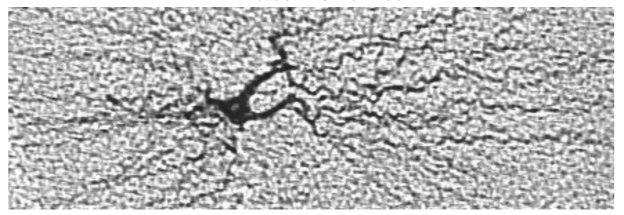
To answer your question, the above is a rendering of a neuron from a rat's hippocampus. The tools we have refined will enable us to model the electrical properties of a dendrite leaving the neuron's cell body. A three-branch model of such a dendrite, traced out with painstaking accuracy, appears in Figure $\PageIndex{2}$.

Figure $\PageIndex{2}$: 3-branch Dendrite Model. Multi-compartment electrical model of a rendered dendrite fiber.

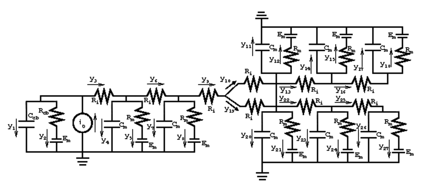
Our multi-compartment model reveals a 3 branch, 10 node, 27 edge structure to the fiber. Note that we have included the Nernst potentials, the nervous impulse as a current source, and the additional leftmost edges depicting stimulus current shunted by the cell body.

We will continue using our previous notation, namely: $R_{i}$ and $R_{m}$ denoting cell body. and membrane resistances, respectively; $\textbf{x}$ representing the vector of potentials $x_{1} \cdots x_{10}$, and $\textbf{x}$ denoting the vector of currents $y_{1} \cdots y_{27}$. Using the typical value for a cell's membrane

$$c = 1(μF/cm^{2}) \nonumber$$

we derive (see variable conventions):

Definition: Capacitance of a Single Compartment

$$C_{m} = 2 \pi a\frac{l}{N}c \nonumber$$

This capacitance is modeled in parallel with the cell's membrane resistance. Additionally, letting $A_{cb}$ denote the cell body's surface area, we recall that its capacitance and resistance are

Definition: Capacitance of a Cell Body

$$C_{cb} = A_{cb} c \nonumber$$

Definition: Resistance of a Cell Body

$$C_{cb} = A_{cb} \rho_{m} \nonumber$$

Applying the Strang Quartet

Step (S1')--Voltage Drops

Let's begin filling out the Strang Quartet. For Step (S1'), we first observe the voltage drops in the figure. Since there are a whopping 27 of them, we include only the first six, which are slightly more than we need to cover all variations in the set:

$$e_{1} = x_{1} \nonumber$$

$$e_{2} = x_{1}-E_{m} \nonumber$$

$$e_{3} = x_{1}-x_{2} \nonumber$$

$$e_{4} = x_{2} \nonumber$$

$$e_{5} = x_{2}-E_{m} \nonumber$$

$$e_{6} = x_{2}-x_{3} \nonumber$$

$$\cdots \nonumber$$

$$e_{27} = x_{10}-E_{m} \nonumber$$

In matrix for, letting $\textbf{b}$ denote the vector of batteries,

$$\begin{array}{ccc} {\textbf{x} = \textbf{b}-A \textbf{x}}&{where}&{\textbf{b} = (-Em) \begin{pmatrix} {0}\\{1}\\{0}\\{0}\\{1}\\{0}\\{0}\\{1}\\{0}\\{0}\\{0}\\{1}\\{0}\\{0}\\{1}\\{0}\\{0}\\{1}\\{0}\\{0}\\{1}\\{0}\\{0}\\{1}\\{0}\\{0}\\{1} \end{pmatrix}} \end{array} \nonumber$$

and

$$A = \begin{pmatrix} {-1}&{0}&{0}&{0}&{0}&{0}&{0}&{0}&{0}&{0}\\ {-1}&{0}&{0}&{0}&{0}&{0}&{0}&{0}&{0}&{0}\\ {-1}&{1}&{0}&{0}&{0}&{0}&{0}&{0}&{0}&{0}\\{0}&{-1}&{0}&{0}&{0}&{0}&{0}&{0}&{0}&{0}\\ {0}&{-1}&{0}&{0}&{0}&{0}&{0}&{0}&{0}&{0}\\ {0}&{-1}&{1}&{0}&{0}&{0}&{0}&{0}&{0}&{0}\\ {0}&{0}&{-1}&{0}&{0}&{0}&{0}&{0}&{0}&{0}\\ {0}&{0}&{-1}&{0}&{0}&{0}&{0}&{0}&{0}&{0}\\ {0}&{0}&{-1}&{1}&{0}&{0}&{0}&{0}&{0}&{0}\\ {0}&{0}&{0}&{1}&{-1}&{0}&{0}&{0}&{0}&{0}\\ {0}&{0}&{0}&{0}&{-1}&{0}&{0}&{0}&{0}&{0}\\ {0}&{0}&{0}&{0}&{-1}&{0}&{0}&{0}&{0}&{0}\\ {0}&{0}&{0}&{0}&{-1}&{1}&{0}&{0}&{0}&{0}\\ {0}&{0}&{0}&{0}&{0}&{-1}&{0}&{0}&{0}&{0}\\ {0}&{0}&{0}&{0}&{0}&{-1}&{0}&{0}&{0}&{0}\\ {0}&{0}&{0}&{0}&{0}&{-1}&{1}&{0}&{0}&{0}\\ {0}&{0}&{0}&{0}&{0}&{0}&{-1}&{0}&{0}&{0}\\ {0}&{0}&{0}&{0}&{0}&{0}&{-1}&{0}&{0}&{0}\\ {0}&{0}&{0}&{-1}&{0}&{0}&{0}&{1}&{0}&{0}\\ {0}&{0}&{0}&{0}&{0}&{0}&{0}&{-1}&{0}&{0}\\ {0}&{0}&{0}&{0}&{0}&{0}&{0}&{-1}&{0}&{0}\\ {0}&{0}&{0}&{0}&{0}&{0}&{0}&{-1}&{1}&{0}\\ {0}&{0}&{0}&{0}&{0}&{0}&{0}&{0}&{-1}&{0}\\ {0}&{0}&{0}&{0}&{0}&{0}&{0}&{0}&{-1}&{0}\\ {0}&{0}&{0}&{0}&{0}&{0}&{0}&{0}&{-1}&{1}\\ {0}&{0}&{0}&{0}&{0}&{0}&{0}&{0}&{0}&{-1}\\ {0}&{0}&{0}&{0}&{0}&{0}&{0}&{0}&{0}&{-1}\\ \end{pmatrix} \nonumber$$

Although our adjacency matrix $A$ is appreciably larger than our previous examples, we have captured the same phenomena as before.

Applying (S2): Ohm's Law Augmented with Voltage-Current Law for Capacitors

Now, recalling Ohm's Law and remembering that the current through a capacitor varies proportionately with the time rate of change of the potential across it, we assemble our vector of currents. As before, we list only enough of the 27 currents to fully characterize the set:

$$y_{1} = C_{cb} \frac{de_{1}}{dt} \nonumber$$

$$y_{2} = \frac{e_{2}}{R_{cb}} \nonumber$$

$$y_{3} = \frac{e_{3}}{R_{i}} \nonumber$$

$$y_{4} = C_{m} \frac{de_{4}}{dt} \nonumber$$

$$y_{5} = \frac{e_{5}}{R_{m}} \nonumber$$

$$\cdots \nonumber$$

$$y_{27} = \frac{e_{27}}{R_{m}} \nonumber$$

In matrix terms, this compiles to

$$\textbf{y} = G \textbf{e}+Cd \textbf{e} dt \nonumber$$

where

Conductance matrix

$$G = \begin{pmatrix} {0}&{0}&{0}&{0}&{0}&{0}&{0}&{0}&{0}&{0}&{0}&{0}&{0}&{0}&{0}&{0}&{0}&{0}&{0}&{0}&{0}&{0}&{0}&{0}&{0}&{0}&{0}\\ {0}&{\frac{1}{R_{cb}}}&{0}&{0}&{0}&{0}&{0}&{0}&{0}&{0}&{0}&{0}&{0}&{0}&{0}&{0}&{0}&{0}&{0}&{0}&{0}&{0}&{0}&{0}&{0}&{0}&{0}\\ {0}&{0}&{\frac{1}{R_{i}}}&{0}&{0}&{0}&{0}&{0}&{0}&{0}&{0}&{0}&{0}&{0}&{0}&{0}&{0}&{0}&{0}&{0}&{0}&{0}&{0}&{0}&{0}&{0}&{0}\\ {0}&{0}&{0}&{0}&{0}&{0}&{0}&{0}&{0}&{0}&{0}&{0}&{0}&{0}&{0}&{0}&{0}&{0}&{0}&{0}&{0}&{0}&{0}&{0}&{0}&{0}&{0}\\ {0}&{0}&{0}&{0}&{\frac{1}{R_{m}}}&{0}&{0}&{0}&{0}&{0}&{0}&{0}&{0}&{0}&{0}&{0}&{0}&{0}&{0}&{0}&{0}&{0}&{0}&{0}&{0}&{0}&{0}\\ {0}&{0}&{0}&{0}&{0}&{\frac{1}{R_{i}}}&{0}&{0}&{0}&{0}&{0}&{0}&{0}&{0}&{0}&{0}&{0}&{0}&{0}&{0}&{0}&{0}&{0}&{0}&{0}&{0}&{0}\\ {0}&{0}&{0}&{0}&{0}&{0}&{0}&{0}&{0}&{0}&{0}&{0}&{0}&{0}&{0}&{0}&{0}&{0}&{0}&{0}&{0}&{0}&{0}&{0}&{0}&{0}&{0}\\ {0}&{0}&{0}&{0}&{0}&{0}&{0}&{\frac{1}{R_{i}}}&{0}&{0}&{0}&{0}&{0}&{0}&{0}&{0}&{0}&{0}&{0}&{0}&{0}&{0}&{0}&{0}&{0}&{0}&{0}\\ {0}&{0}&{0}&{0}&{0}&{0}&{0}&{0}&{\frac{1}{R_{i}}}&{0}&{0}&{0}&{0}&{0}&{0}&{0}&{0}&{0}&{0}&{0}&{0}&{0}&{0}&{0}&{0}&{0}&{0}\\ {0}&{0}&{0}&{0}&{0}&{0}&{0}&{0}&{0}&{\frac{1}{R_{i}}}&{0}&{0}&{0}&{0}&{0}&{0}&{0}&{0}&{0}&{0}&{0}&{0}&{0}&{0}&{0}&{0}&{0}\\ {0}&{0}&{0}&{0}&{0}&{0}&{0}&{0}&{0}&{0}&{0}&{0}&{0}&{0}&{0}&{0}&{0}&{0}&{0}&{0}&{0}&{0}&{0}&{0}&{0}&{0}&{0}\\ {0}&{0}&{0}&{0}&{0}&{0}&{0}&{0}&{0}&{0}&{0}&{\frac{1}{R_{m}}}&{0}&{0}&{0}&{0}&{0}&{0}&{0}&{0}&{0}&{0}&{0}&{0}&{0}&{0}&{0}\\ {0}&{0}&{0}&{0}&{0}&{0}&{0}&{0}&{0}&{0}&{0}&{0}&{\frac{1}{R_{i}}}&{0}&{0}&{0}&{0}&{0}&{0}&{0}&{0}&{0}&{0}&{0}&{0}&{0}&{0}\\ {0}&{0}&{0}&{0}&{0}&{0}&{0}&{0}&{0}&{0}&{0}&{0}&{0}&{0}&{0}&{0}&{0}&{0}&{0}&{0}&{0}&{0}&{0}&{0}&{0}&{0}&{0}\\ {0}&{0}&{0}&{0}&{0}&{0}&{0}&{0}&{0}&{0}&{0}&{0}&{0}&{0}&{\frac{1}{R_{m}}}&{0}&{0}&{0}&{0}&{0}&{0}&{0}&{0}&{0}&{0}&{0}&{0}\\ {0}&{0}&{0}&{0}&{0}&{0}&{0}&{0}&{0}&{0}&{0}&{0}&{0}&{0}&{0}&{\frac{1}{R_{i}}}&{0}&{0}&{0}&{0}&{0}&{0}&{0}&{0}&{0}&{0}&{0}\\ {0}&{0}&{0}&{0}&{0}&{0}&{0}&{0}&{0}&{0}&{0}&{0}&{0}&{0}&{0}&{0}&{0}&{0}&{0}&{0}&{0}&{0}&{0}&{0}&{0}&{0}&{0}\\ {0}&{0}&{0}&{0}&{0}&{0}&{0}&{0}&{0}&{0}&{0}&{0}&{0}&{0}&{0}&{0}&{0}&{\frac{1}{R_{m}}}&{0}&{0}&{0}&{0}&{0}&{0}&{0}&{0}&{0}\\ {0}&{0}&{0}&{0}&{0}&{0}&{0}&{0}&{0}&{0}&{0}&{0}&{0}&{0}&{0}&{0}&{0}&{0}&{\frac{1}{R_{i}}}&{0}&{0}&{0}&{0}&{0}&{0}&{0}&{0}\\ {0}&{0}&{0}&{0}&{0}&{0}&{0}&{0}&{0}&{0}&{0}&{0}&{0}&{0}&{0}&{0}&{0}&{0}&{0}&{0}&{0}&{0}&{0}&{0}&{0}&{0}&{0}\\ {0}&{0}&{0}&{0}&{0}&{0}&{0}&{0}&{0}&{0}&{0}&{0}&{0}&{0}&{0}&{0}&{0}&{0}&{0}&{0}&{\frac{1}{R_{m}}}&{0}&{0}&{0}&{0}&{0}&{0}\\ {0}&{0}&{0}&{0}&{0}&{0}&{0}&{0}&{0}&{0}&{0}&{0}&{0}&{0}&{0}&{0}&{0}&{0}&{0}&{0}&{0}&{\frac{1}{R_{i}}}&{0}&{0}&{0}&{0}&{0}\\ {0}&{0}&{0}&{0}&{0}&{0}&{0}&{0}&{0}&{0}&{0}&{0}&{0}&{0}&{0}&{0}&{0}&{0}&{0}&{0}&{0}&{0}&{0}&{0}&{0}&{0}&{0}\\ {0}&{0}&{0}&{0}&{0}&{0}&{0}&{0}&{0}&{0}&{0}&{0}&{0}&{0}&{0}&{0}&{0}&{0}&{0}&{0}&{0}&{0}&{0}&{\frac{1}{R_{m}}}&{0}&{0}&{0}\\ {0}&{0}&{0}&{0}&{0}&{0}&{0}&{0}&{0}&{0}&{0}&{0}&{0}&{0}&{0}&{0}&{0}&{0}&{0}&{0}&{0}&{0}&{0}&{0}&{\frac{1}{R_{i}}}&{0}&{0}\\ {0}&{0}&{0}&{0}&{0}&{0}&{0}&{0}&{0}&{0}&{0}&{0}&{0}&{0}&{0}&{0}&{0}&{0}&{0}&{0}&{0}&{0}&{0}&{0}&{0}&{0}&{0}\\ {0}&{0}&{0}&{0}&{0}&{0}&{0}&{0}&{0}&{0}&{0}&{0}&{0}&{0}&{0}&{0}&{0}&{0}&{0}&{0}&{0}&{0}&{0}&{0}&{0}&{0}&{\frac{1}{R_{m}}} \end{pmatrix} \nonumber$$

and

Capacitance matrix

$$C = \begin{pmatrix} {C_{cb}}&{0}&{0}&{0}&{0}&{0}&{0}&{0}&{0}&{0}&{0}&{0}&{0}&{0}&{0}&{0}&{0}&{0}&{0}&{0}&{0}&{0}&{0}&{0}&{0}&{0}&{0}\\ {0}&{0}&{0}&{0}&{0}&{0}&{0}&{0}&{0}&{0}&{0}&{0}&{0}&{0}&{0}&{0}&{0}&{0}&{0}&{0}&{0}&{0}&{0}&{0}&{0}&{0}&{0}\\ {0}&{0}&{0}&{0}&{0}&{0}&{0}&{0}&{0}&{0}&{0}&{0}&{0}&{0}&{0}&{0}&{0}&{0}&{0}&{0}&{0}&{0}&{0}&{0}&{0}&{0}&{0}\\ {0}&{0}&{0}&{C_{m}}&{0}&{0}&{0}&{0}&{0}&{0}&{0}&{0}&{0}&{0}&{0}&{0}&{0}&{0}&{0}&{0}&{0}&{0}&{0}&{0}&{0}&{0}&{0}\\ {0}&{0}&{0}&{0}&{0}&{0}&{0}&{0}&{0}&{0}&{0}&{0}&{0}&{0}&{0}&{0}&{0}&{0}&{0}&{0}&{0}&{0}&{0}&{0}&{0}&{0}&{0}\\ {0}&{0}&{0}&{0}&{0}&{0}&{0}&{0}&{0}&{0}&{0}&{0}&{0}&{0}&{0}&{0}&{0}&{0}&{0}&{0}&{0}&{0}&{0}&{0}&{0}&{0}&{0}\\ {0}&{0}&{0}&{0}&{0}&{0}&{C_{m}}&{0}&{0}&{0}&{0}&{0}&{0}&{0}&{0}&{0}&{0}&{0}&{0}&{0}&{0}&{0}&{0}&{0}&{0}&{0}&{0}\\ {0}&{0}&{0}&{0}&{0}&{0}&{0}&{0}&{0}&{0}&{0}&{0}&{0}&{0}&{0}&{0}&{0}&{0}&{0}&{0}&{0}&{0}&{0}&{0}&{0}&{0}&{0}\\ {0}&{0}&{0}&{0}&{0}&{0}&{0}&{0}&{0}&{0}&{0}&{0}&{0}&{0}&{0}&{0}&{0}&{0}&{0}&{0}&{0}&{0}&{0}&{0}&{0}&{0}&{0}\\ {0}&{0}&{0}&{0}&{0}&{0}&{0}&{0}&{0}&{0}&{0}&{0}&{0}&{0}&{0}&{0}&{0}&{0}&{0}&{0}&{0}&{0}&{0}&{0}&{0}&{0}&{0}\\ {0}&{0}&{0}&{0}&{0}&{0}&{0}&{0}&{0}&{0}&{C_{m}}&{0}&{0}&{0}&{0}&{0}&{0}&{0}&{0}&{0}&{0}&{0}&{0}&{0}&{0}&{0}&{0}\\ {0}&{0}&{0}&{0}&{0}&{0}&{0}&{0}&{0}&{0}&{0}&{0}&{0}&{0}&{0}&{0}&{0}&{0}&{0}&{0}&{0}&{0}&{0}&{0}&{0}&{0}&{0}\\ {0}&{0}&{0}&{0}&{0}&{0}&{0}&{0}&{0}&{0}&{0}&{0}&{0}&{0}&{0}&{0}&{0}&{0}&{0}&{0}&{0}&{0}&{0}&{0}&{0}&{0}&{0}\\ {0}&{0}&{0}&{0}&{0}&{0}&{0}&{0}&{0}&{0}&{0}&{0}&{0}&{C_{m}}&{0}&{0}&{0}&{0}&{0}&{0}&{0}&{0}&{0}&{0}&{0}&{0}&{0}\\ {0}&{0}&{0}&{0}&{0}&{0}&{0}&{0}&{0}&{0}&{0}&{0}&{0}&{0}&{0}&{0}&{0}&{0}&{0}&{0}&{0}&{0}&{0}&{0}&{0}&{0}&{0}\\ {0}&{0}&{0}&{0}&{0}&{0}&{0}&{0}&{0}&{0}&{0}&{0}&{0}&{0}&{0}&{0}&{0}&{0}&{0}&{0}&{0}&{0}&{0}&{0}&{0}&{0}&{0}\\ {0}&{0}&{0}&{0}&{0}&{0}&{0}&{0}&{0}&{0}&{0}&{0}&{0}&{0}&{0}&{0}&{C_{m}}&{0}&{0}&{0}&{0}&{0}&{0}&{0}&{0}&{0}&{0}\\ {0}&{0}&{0}&{0}&{0}&{0}&{0}&{0}&{0}&{0}&{0}&{0}&{0}&{0}&{0}&{0}&{0}&{0}&{0}&{0}&{0}&{0}&{0}&{0}&{0}&{0}&{0}\\ {0}&{0}&{0}&{0}&{0}&{0}&{0}&{0}&{0}&{0}&{0}&{0}&{0}&{0}&{0}&{0}&{0}&{0}&{0}&{0}&{0}&{0}&{0}&{0}&{0}&{0}&{0}\\ {0}&{0}&{0}&{0}&{0}&{0}&{0}&{0}&{0}&{0}&{0}&{0}&{0}&{0}&{0}&{0}&{0}&{0}&{0}&{C_{m}}&{0}&{0}&{0}&{0}&{0}&{0}&{0}\\ {0}&{0}&{0}&{0}&{0}&{0}&{0}&{0}&{0}&{0}&{0}&{0}&{0}&{0}&{0}&{0}&{0}&{0}&{0}&{0}&{0}&{0}&{0}&{0}&{0}&{0}&{0}\\ {0}&{0}&{0}&{0}&{0}&{0}&{0}&{0}&{0}&{0}&{0}&{0}&{0}&{0}&{0}&{0}&{0}&{0}&{0}&{0}&{0}&{0}&{0}&{0}&{0}&{0}&{0}\\ {0}&{0}&{0}&{0}&{0}&{0}&{0}&{0}&{0}&{0}&{0}&{0}&{0}&{0}&{0}&{0}&{0}&{0}&{0}&{0}&{0}&{0}&{C_{m}}&{0}&{0}&{0}&{0}\\ {0}&{0}&{0}&{0}&{0}&{0}&{0}&{0}&{0}&{0}&{0}&{0}&{0}&{0}&{0}&{0}&{0}&{0}&{0}&{0}&{0}&{0}&{0}&{0}&{0}&{0}&{0}\\ {0}&{0}&{0}&{0}&{0}&{0}&{0}&{0}&{0}&{0}&{0}&{0}&{0}&{0}&{0}&{0}&{0}&{0}&{0}&{0}&{0}&{0}&{0}&{0}&{0}&{0}&{0}\\ {0}&{0}&{0}&{0}&{0}&{0}&{0}&{0}&{0}&{0}&{0}&{0}&{0}&{0}&{0}&{0}&{0}&{0}&{0}&{0}&{0}&{0}&{0}&{0}&{0}&{C_{m}}&{0}\\ {0}&{0}&{0}&{0}&{0}&{0}&{0}&{0}&{0}&{0}&{0}&{0}&{0}&{0}&{0}&{0}&{0}&{0}&{0}&{0}&{0}&{0}&{0}&{0}&{0}&{0}&{0} \end{pmatrix} \nonumber$$

Step (S3): Applying Kirchoff's Law

Our next step is to write out the equations for Kirchoff's Current Law. We see:

$$i_{0}-y_{1}-y_{2}-y_{3} = 0 \nonumber$$

$$y_{3}-y_{4}-y_{5}-y_{6} = 0 \nonumber$$

$$y_{6}-y_{7}-y_{8}-y_{9} = 0 \nonumber$$

$$y_{9}-y_{10}-y_{19} = 0 \nonumber$$

$$y_{10}-y_{11}-y_{12}-y_{13} = 0 \nonumber$$

$$y_{13}-y_{14}-y_{15}-y_{16} = 0 \nonumber$$

$$y_{16}-y_{17}-y_{18}-y_{19} = 0 \nonumber$$

$$y_{19}-y_{20}-y_{21}-y_{22} = 0 \nonumber$$

$$y_{22}-y_{23}-y_{24}-y_{25} = 0 \nonumber$$

$$y_{25}-y_{26}-y_{27} = 0 \nonumber$$

Since the $B$ coefficient matrix we'd form here is equal to $A^{T}$, we can say in matrix terms:

$$A^{T} \textbf{y} = -\textbf{f} \nonumber$$

where the vector $\textbf{f}$ is composed of $f_{1} = i_{0}$ and $f_{2} \cdots 27 = 0$

Step (S4): Stirring the Ingredients Together

Step (S4) directs us to assemble our previous toils together into a final equation, which we will then endeavor to solve. Using the process derived in the dynamic Strang module, we arrive at the equation

$$A^{T}CA \frac{d \textbf{x}}{dt}+A^{T}GA \textbf{x} = A^{T}G \textbf{b}+\textbf{f}+A^{T}C \frac{d\textbf{b}}{dt} \nonumber$$

which is the general form for RC circuit potential equations. As we have mentioned, this equation presumes knowledge of the initial value of each of the potentials, $\textbf{x}(⁢0) = X$.

Observing our circuit, and letting $\frac{1}{R_{foo}} = G_{foo}$, we calculate the necessary quantities to fill out Equation's pieces (for these calculations, see dendrite.m):

$$A^{T}CA = \begin{pmatrix} {C_{cb}}&{0}&{0}&{0}&{0}&{0}&{0}&{0}&{0}&{0}\\ {0}&{C_{m}}&{0}&{0}&{0}&{0}&{0}&{0}&{0}&{0}\\ {0}&{0}&{C_{m}}&{0}&{0}&{0}&{0}&{0}&{0}&{0}\\ {0}&{0}&{0}&{C_{m}}&{0}&{0}&{0}&{0}&{0}&{0}\\ {0}&{0}&{0}&{0}&{C_{m}}&{0}&{0}&{0}&{0}&{0}\\ {0}&{0}&{0}&{0}&{0}&{C_{m}}&{0}&{0}&{0}&{0}\\ {0}&{0}&{0}&{0}&{0}&{0}&{C_{m}}&{0}&{0}&{0}\\ {0}&{0}&{0}&{0}&{0}&{0}&{0}&{C_{m}}&{0}&{0}\\ {0}&{0}&{0}&{0}&{0}&{0}&{0}&{0}&{C_{m}}&{0}\\ {0}&{0}&{0}&{0}&{0}&{0}&{0}&{0}&{0}&{C_{m}} \end{pmatrix} \nonumber$$

$$A^{T}GA = \begin{pmatrix} {G_{i}+G_{cb}}&{-G_{i}}&{0}&{0}&{0}&{0}&{0}&{0}&{0}&{0}\\ {-G_{i}}&{2G_{i}+G_{m}}&{-G_{i}}&{0}&{0}&{0}&{0}&{0}&{0}&{0}\\ {0}&{-G_{i}}&{2G_{i}+G_{m}}&{-G_{i}}&{0}&{0}&{0}&{0}&{0}&{0}\\ {0}&{0}&{-G_{i}}&{3G_{i}}&{-G_{i}}&{0}&{0}&{-G_{i}}&{0}&{0}\\ {0}&{0}&{0}&{-G_{i}}&{2G_{i}+G_{m}}&{-G_{i}}&{0}&{0}&{0}&{0}\\ {0}&{0}&{0}&{0}&{-G_{i}}&{2G_{i}+G_{m}}&{-G_{i}}&{0}&{0}&{0}\\ {0}&{0}&{0}&{0}&{0}&{-G_{i}}&{G_{i}+G_{m}}&{0}&{0}&{0}\\ {0}&{0}&{0}&{-G_{i}}&{0}&{0}&{0}&{2G_{i}+G_{m}}&{-G_{i}}&{0}\\ {0}&{0}&{0}&{0}&{0}&{0}&{0}&{-G_{i}}&{2G_{i}+G_{m}}&{-G_{i}}\\ {0}&{0}&{0}&{0}&{0}&{0}&{0}&{0}&{-G_{i}}&{G_{i}+G_{m}} \end{pmatrix} \nonumber$$

$$A^{T}G \textbf{b} = E_{m} \begin{pmatrix} {G_{cb}}\\ {G_{m}}\\ {G_{m}}\\ {0}\\ {G_{m}}\\ {G_{m}}\\ {G_{m}}\\ {G_{m}}\\ {G_{m}}\\ {G_{m}} \end{pmatrix} \nonumber$$

$$A^{T}C \frac{d \textbf{b}}{dt} = \textbf{0} \nonumber$$

and an initial (rest) potential of

$$\textbf{x}(0) = E_{m} \begin{pmatrix} {1}\\ {1}\\ {1}\\ {1}\\ {1}\\ {1}\\ {1}\\ {1}\\ {1}\\ {1} \end{pmatrix} \nonumber$$

Applying the Backward-Euler Method

Since our system is so large, the Backward-Euler method is the best path to a solution. Looking at the matrix $A^{T}CA$ we observe that it is singular and therefore non-invertible. This singularity arises from the node connecting the three branches of the fiber and prevents us from using the simple equation $\textbf{x}' = B \textbf{x}+\textbf{g}$, we used in earlier Backward-Euler-ings. However, we will see that a modest generalization to our previous form yields Equation:

$$D \textbf{x}' = E\textbf{x}+\textbf{g} \nonumber$$

capturing the form of our system and allowing us to solve for $\textbf{x}⁢(t)$ Equation as follows:

$$D \textbf{x}' = E\textbf{x}+\textbf{g} \nonumber$$

$$D \frac{\tilde{x}(t)-\tilde{x}(t-dt)}{dt} = E\tilde{x}(t)+\textbf{g} \nonumber$$

$$(D-Edt) \tilde{x}(t) = D\tilde{x}(t-dt)+\textbf{g}dt \nonumber$$

$$\tilde{x}(t) = (D-Edt)^{-1}(\tilde{x}(t-dt)+\textbf{g}dt) \nonumber$$

where in our case

$$D = A^{T}CA \nonumber$$

$$E = -(A^{T}GA) \nonumber$$

$$\textbf{g} = A^{T}G \textbf{b}+\textbf{f} \nonumber$$ .

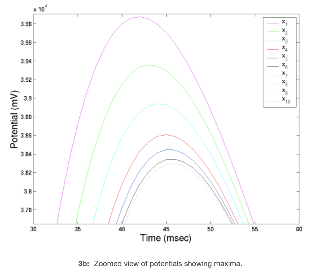
This method is implemented in dendrite.m with typical cell dimensions and resistivity properties, yielding the following graph of potentials.

Graph of Dendrite Potentials

Figure 3.