9.1: The Matrix of a Linear Transformation

Let \(T : V \to W\) be a linear transformation where \(dim \;V = n\) and \(dim \;W = m\). The aim in this section is to describe the action of \(T\) as multiplication by an \(m \times n\) matrix \(A\). The idea is to convert a vector \(\mathbf{v}\) in \(V\) into a column in \(\mathbb{R}^n\), multiply that column by \(A\) to get a column in \(\mathbb{R}^m\), and convert this column back to get \(T(\mathbf{v})\) in \(W\).

Converting vectors to columns is a simple matter, but one small change is needed. Up to now the order of the vectors in a basis has been of no importance. However, in this section, we shall speak of an ordered basis \(\{\mathbf{b}_{1}, \mathbf{b}_{2}, \dots, \mathbf{b}_{n}\}\), which is just a basis where the order in which the vectors are listed is taken into account. Hence \(\{\mathbf{b}_{2}, \mathbf{b}_{1}, \mathbf{b}_{3}\}\) is a different ordered basis from \(\{\mathbf{b}_{1}, \mathbf{b}_{2}, \mathbf{b}_{3}\}\).

If \(B = \{\mathbf{b}_{1}, \mathbf{b}_{2}, \dots, \mathbf{b}_{n}\}\) is an ordered basis in a vector space \(V\), and if

\[\mathbf{v} = v_1\mathbf{b}_1 + v_2\mathbf{b}_2 + \cdots + v_n\mathbf{b}_n, \quad v_i \in \mathbb{R} \nonumber \]

is a vector in \(V\), then the (uniquely determined) numbers \(v_{1}, v_{2}, \dots, v_{n}\) are called the coordinates of \(\mathbf{v}\) with respect to the basis \(B\).

Definition: Coordinate Vector \(C_B(\mathbf{v})\) of \(\mathbf{v}\) for a basis \(B\)

The coordinate vector of \(\mathbf{v}\) with respect to \(B\) is defined to be

\[C_B(\mathbf{v})= (v_1\mathbf{b}_1 + v_2\mathbf{b}_2 + \cdots + v_n\mathbf{b}_n) = \left[ \begin{array}{c} v_1 \\ v_2 \\ \vdots \\ v_n \end{array} \right] \nonumber \]

The reason for writing \(C_{B}(\mathbf{v})\) as a column instead of a row will become clear later. Note that \(C_{B}(\mathbf{b}_{i}) = \mathbf{e}_{i}\) is column \(i\) of \(I_{n}\).

Example \(\PageIndex{1}\)

The coordinate vector for \(\mathbf{v} = (2, 1, 3)\) with respect to the ordered basis \(B = \{(1, 1, 0), (1, 0, 1), (0, 1, 1)\}\) of \(\mathbb{R}^3\) is \(C_B(\mathbf{v}) = \left[ \begin{array}{c} 0 \\ 2 \\ 1 \end{array} \right]\) because

\[\mathbf{v} = (2, 1, 3) = 0(1, 1, 0) + 2(1, 0, 1) + 1(0, 1, 1) \nonumber \]

Theorem \(\PageIndex{1}\)

If \(V\) has dimension \(n\) and \(B = \{\mathbf{b}_{1}, \mathbf{b}_{2}, \dots, \mathbf{b}_{n}\}\) is any ordered basis of \(V\), the coordinate transformation \(C_{B} : V \to \mathbb{R}^n\) is an isomorphism. In fact, \(C_B^{-1} : \mathbb{R}^n \to V\) is given by

\[C_B^{-1} \left[ \begin{array}{c} v_1 \\ v_2 \\ \vdots \\ v_n \end{array} \right] = v_1\mathbf{b}_1 + v_2\mathbf{b}_2 + \cdots + v_n\mathbf{b}_n \quad \mbox{ for all } \quad \left[ \begin{array}{c} v_1 \\ v_2 \\ \vdots \\ v_n \end{array} \right] \mbox{ in } \mathbb{R}^n. \nonumber \]

Proof

The verification that \(C_{B}\) is linear is Exercise 9.1.13. If \(T : \mathbb{R}^n \to V\) is the map denoted \(C_B^{-1}\) in the theorem, one verifies (Exercise 9.1.13) that \(TC_{B} = 1_{V}\) and \(C_BT = 1_{\mathbb{R}^n}\). Note that \(C_{B}(\mathbf{b}_{j})\) is column \(j\) of the identity matrix, so \(C_{B}\) carries the basis \(B\) to the standard basis of \(\mathbb{R}^n\), proving again that it is an isomorphism (Theorem 7.3.1)

Now let \(T : V \to W\) be any linear transformation where \(dim \;V = n\) and \(dim \;W = m\), and let \(B = \{\mathbf{b}_{1}, \mathbf{b}_{2}, \dots, \mathbf{b}_{n}\}\) and \(D\) be ordered bases of \(V\) and \(W\), respectively. Then \(C_{B} : V \to \mathbb{R}^n\) and \(C_{D} : W \to \mathbb{R}^m\) are isomorphisms and we have the situation shown in the diagram where \(A\) is an \(m \times n\) matrix (to be determined).

In fact, the composite

\[C_DTC_B^{-1} : \mathbb{R}^n \to \mathbb{R}^m \mbox{ is a linear transformation} \nonumber \]

so Theorem 2.6.2 shows that a unique \(m \times n\) matrix \(A\) exists such that

\[C_DTC_B^{-1} = T_A, \quad \mbox{ equivalently } C_DT = T_AC_B \nonumber \]

\(T_{A}\) acts by left multiplication by \(A\), so this latter condition is

\[C_D [T(\mathbf{v})] = AC_B(\mathbf{v}) \mbox{ for all } \mathbf{v} \mbox{ in } V \nonumber \]

This requirement completely determines \(A\). Indeed, the fact that \(C_{B}(\mathbf{b}_{j})\) is column \(j\) of the identity matrix gives

\[\mbox{column } j \mbox{ of } A = AC_B(\mathbf{b}_j) = C_D[T(\mathbf{b}_j)] \nonumber \]

for all \(j\). Hence, in terms of its columns,

\[A = \left[ \begin{array}{cccc} C_D[T(\mathbf{b}_1)] & C_D[T(\mathbf{b}_2)] & \cdots & C_D[T(\mathbf{b}_n)] \end{array} \right] \nonumber \]

Definition: Matrix \(M_{DB}(T)\) of \(T : V \to W\) for bases \(D\) and \(B\)

This is called the matrix of \(T\) corresponding to the ordered bases \(B\) and \(D\), and we use the following notation:

\[M_{DB}(T) = \left[ \begin{array}{cccc} C_D[T(\mathbf{b}_1)] & C_D[T(\mathbf{b}_2)] & \cdots & C_D[T(\mathbf{b}_n)] \end{array}\right] \nonumber \]

This discussion is summarized in the following important theorem.

Theorem \(\PageIndex{2}\)

Let \(T : V \to W\) be a linear transformation where \(dim \;V = n\) and \(dim \;W = m\), and let \(B = \{\mathbf{b}_{1}, \dots, \mathbf{b}_{n}\}\) and \(D\) be ordered bases of \(V\) and \(W\), respectively. Then the matrix \(M_{DB}(T)\) just given is the unique \(m \times n\) matrix \(A\) that satisfies

\[C_DT = T_AC_B \nonumber \]

Hence the defining property of \(M_{DB}(T)\) is

\[C_D[T(\mathbf{v})] = M_{DB}(T)C_B(\mathbf{v}) \mbox{ for all } \mathbf{v} \mbox{ in } V \nonumber \]

The matrix \(M_{DB}(T)\) is given in terms of its columns by

\[M_{DB}(T) = \left[ \begin{array}{cccc} C_D[T(\mathbf{b}_1)] & C_D[T(\mathbf{b}_2)] & \cdots & C_D[T(\mathbf{b}_n)] \end{array}\right] \nonumber \]

The fact that \(T = C_D^{-1}T_AC_B\) means that the action of \(T\) on a vector \(\mathbf{v}\) in \(V\) can be performed by first taking coordinates (that is, applying \(C_{B}\) to \(\mathbf{v}\)), then multiplying by \(A\) (applying \(T_{A}\)), and finally converting the resulting \(m\)-tuple back to a vector in \(W\) (applying \(C_D^{-1}\)).

Example \(\PageIndex{2}\)

Define \(T :\|{P}_{2} \to \mathbb{R}^2\) by \(T(a + bx + cx^{2}) = (a + c, b - a - c)\) for all polynomials \(a + bx + cx^{2}\). If \(B = \{\mathbf{b}_{1}, \mathbf{b}_{2}, \mathbf{b}_{3}\}\) and \(D = \{\mathbf{d}_{1}, \mathbf{d}_{2}\}\) where

\[\mathbf{b}_1 = 1, \mathbf{b}_2 = x, \mathbf{b}_3 = x^2 \quad \mbox{ and } \quad \mathbf{d}_1 = (1, 0), \mathbf{d}_2 = (0, 1) \nonumber \]

compute \(M_{DB}(T)\) and verify Theorem 9.1.2.

Solution

We have \(T(\mathbf{b}_{1}) = \mathbf{d}_{1} - \mathbf{d}_{2}\), \(T(\mathbf{b}_{2}) = \mathbf{d}_{2}\), and \(T(\mathbf{b}_{3}) = \mathbf{d}_{1} - \mathbf{d}_{2}\). Hence

\[M_{DB}(T) = \left[ \begin{array}{ccc} C_D[T(\mathbf{b}_1)] & C_D[T(\mathbf{b}_2)] & C_D[T(\mathbf{b}_n)] \end{array}\right] = \left[ \begin{array}{rrr} 1 & 0 & 1 \\ -1 & 1 & -1 \end{array} \right] \nonumber \]

If \(\mathbf{v} = a + bx + cx^{2} = a\mathbf{b}_{1} + b\mathbf{b}_{2} + c\mathbf{b}_{3}\), then \(T(\mathbf{v}) = (a + c)\mathbf{d}_{1} + (b - a - c)\mathbf{d}_{2}\), so

\[C_D[T(\mathbf{v})] = \left[ \begin{array}{c} a + c \\ b - a - c \end{array} \right] = \left[ \begin{array}{rrr} 1 & 0 & 1 \\ -1 & 1 & -1 \end{array} \right] \left[ \begin{array}{c} a \\ b \\ c \end{array} \right] = M_{DB}(T)C_B(\mathbf{v}) \nonumber \]

as Theorem 9.1.2 asserts.

The next example shows how to determine the action of a transformation from its matrix.

Example \(\PageIndex{3}\)

Suppose \(T :\|{M}_{22}(\mathbb{R}) \to \mathbb{R}^3\) is linear with matrix \(M_{DB}(T) = \left[ \begin{array}{rrrr} 1 & -1 & 0 & 0 \\ 0 & 1 & -1 & 0 \\ 0 & 0 & 1 & -1 \end{array} \right]\) where

\[B = \left\{ \left[ \begin{array}{cc} 1 & 0 \\ 0 & 0 \end{array} \right], \left[ \begin{array}{cc} 0 & 1 \\ 0 & 0 \end{array} \right], \left[ \begin{array}{cc} 0 & 0 \\ 1 & 0 \end{array} \right], \left[ \begin{array}{cc} 0 & 0 \\ 0 & 1 \end{array} \right] \right\} \mbox{ and } D = \{(1, 0, 0), (0, 1, 0), (0, 0, 1)\} \nonumber \]

Compute \(T(\mathbf{v})\) where \(\mathbf{v} = \left[ \begin{array}{cc} a & b \\ c & d \end{array} \right]\).

Solution

The idea is to compute \(C_{D}[T(\mathbf{v})]\) first, and then obtain \(T(\mathbf{v})\). We have

\[C_D[T(\mathbf{v})] = M_{DB}(T)C_B(\mathbf{v}) = \left[ \begin{array}{rrrr} 1 & -1 & 0 & 0 \\ 0 & 1 & -1 & 0 \\ 0 & 0 & 1 & -1 \end{array} \right] \left[ \begin{array}{c} a \\ b \\ c \\ d \end{array} \right] = \left[ \begin{array}{c} a - b \\ b - c \\ c - d \end{array} \right] \nonumber \]

\[\begin{aligned} \mbox{Hence } T(\mathbf{v}) & = (a - b)(1, 0, 0) + (b - c)(0, 1, 0) + (c - d)(0, 0, 1) \\ & = (a - b, b - c, c - d)\end{aligned} \nonumber \]

The next two examples will be referred to later.

Example \(\PageIndex{4}\)

Let \(A\) be an \(m \times n\) matrix, and let \(T_{A} : \mathbb{R}^n \to \mathbb{R}^m\) be the matrix transformation induced by \(A : T_{A}(\mathbf{x}) = A\mathbf{x}\) for all columns \(\mathbf{x}\) in \(\mathbb{R}^n\). If \(B\) and \(D\) are the standard bases of \(\mathbb{R}^n\) and \(\mathbb{R}^m\), respectively (ordered as usual), then

\[M_{DB}(T_A) = A \nonumber \]

In other words, the matrix of \(T_{A}\) corresponding to the standard bases is \(A\) itself.

Solution

Write \(B = \{\mathbf{e}_{1}, \dots, \mathbf{e}_{n}\}\). Because \(D\) is the standard basis of \(\mathbb{R}^m\), it is easy to verify that \(C_{D}(\mathbf{y}) = \mathbf{y}\) for all columns \(\mathbf{y}\) in \(\mathbb{R}^m\). Hence

\[M_{DB}(T_A) = \left[ \begin{array}{cccc} T_A(\mathbf{e}_1) & T_A(\mathbf{e}_2) & \cdots & T_A(\mathbf{e}_n) \end{array} \right] = \left[ \begin{array}{cccc} A\mathbf{e}_1 & A\mathbf{e}_2 & \cdots & A\mathbf{e}_n \end{array} \right] = A \nonumber \]

because \(A\mathbf{e}_{j}\) is the \(j\)th column of \(A\).

Example \(\PageIndex{5}\)

Let \(V\) and \(W\) have ordered bases \(B\) and \(D\), respectively. Let \(dim \;V = n\).

1. The identity transformation \(1_{V} : V \to V\) has matrix \(M_{BB}(1_{V}) = I_{n}\).
2. The zero transformation \(0 : V \to W\) has matrix \(M_{DB}(0) = 0\).

The first result in Example 9.1.5 is false if the two bases of \(V\) are not equal. In fact, if \(B\) is the standard basis of \(\mathbb{R}^n\), then the basis \(D\) of \(\mathbb{R}^n\) can be chosen so that \(M_{DB}(1_{\mathbb{R}^n})\) turns out to be any invertible matrix we wish (Exercise 9.1.14).

The next two theorems show that composition of linear transformations is compatible with multiplication of the corresponding matrices.

Theorem \(\PageIndex{3}\)

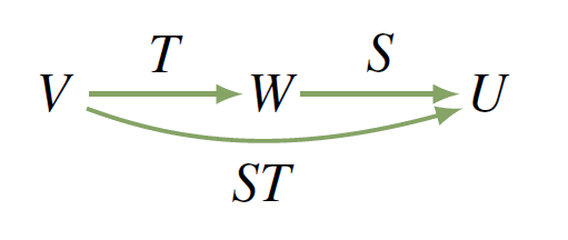
Let \(V \stackrel{T}{\to} W \stackrel{S}{\to} U\) be linear transformations and let \(B\), \(D\), and \(E\) be finite ordered bases of \(V\), \(W\), and \(U\), respectively. Then

\[M_{EB}(ST) = M_{ED}(S) \cdot M_{DB}(T) \nonumber \]

Proof

We use the property in Theorem 9.1.2 three times. If \(\mathbf{v}\) is in \(V\),

\[M_{ED}(S)M_{DB}(T)C_B(\mathbf{v}) = M_{ED}(S)C_D[T(\mathbf{v})] = C_E[ST(\mathbf{v})] = M_{EB}(ST)C_B(\mathbf{v}) \nonumber \]

If \(B = \{\mathbf{e}_{1}, \dots, \mathbf{e}_{n}\}\), then \(C_{B}(\mathbf{e}_{j})\) is column \(j\) of \(I_{n}\). Hence taking \(\mathbf{v} = \mathbf{e}_{j}\) shows that \(M_{ED}(S)M_{DB}(T)\) and \(M_{EB}(ST)\) have equal \(j\)th columns. The theorem follows.

Theorem \(\PageIndex{4}\)

Let \(T : V \to W\) be a linear transformation, where \(dim \;V = dim \;W = n\). The following are equivalent.

1. \(T\) is an isomorphism.
2. \(M_{DB}(T)\) is invertible for all ordered bases \(B\) and \(D\) of \(V\) and \(W\).
3. \(M_{DB}(T)\) is invertible for some pair of ordered bases \(B\) and \(D\) of \(V\) and \(W\).

When this is the case, \([M_{DB}(T)]^{-1} = M_{BD}(T^{-1})\).

Proof

(1) \(\Rightarrow\) (2). We have \(V \stackrel{T}{\to} W \stackrel{T^{-1}}{\to} V\), so Theorem 9.1.3 and Example 9.1.5 give

\[M_{BD}(T^{-1})M_{DB}(T) = M_{BB}(T^{-1}T) = M_{BB}(1v) = I_n \nonumber \]

Similarly, \(M_{DB}(T)M_{BD}(T^{-1}) = I_{n}\), proving (2) (and the last statement in the theorem).

(2) \(\Rightarrow\) (3). This is clear.

(3) \(\Rightarrow\) (1). Suppose that \(T_{DB}(T)\) is invertible for some bases \(B\) and \(D\) and, for convenience, write \(A = M_{DB}(T)\). Then we have \(C_{D}T = T_{A}C_{B}\) by Theorem 9.1.2, so

\[T = (C_D)^{-1}T_AC_B \nonumber \]

by Theorem 9.1.1 where \((C_{D})^{-1}\) and \(C_{B}\) are isomorphisms. Hence (1) follows if we can demonstrate that \(T_{A} : \mathbb{R}^n \to \mathbb{R}^n\) is also an isomorphism. But \(A\) is invertible by (3) and one verifies that \(T_AT_{A^{-1}} = 1_{\mathbb{R}^n} = T_{A^{-1}}T_A\). So \(T_{A}\) is indeed invertible (and \((T_{A})^{-1} = T_{A^{-1}}\)).

In Section 7.2 we defined the \(rank \;\) of a linear transformation \(T : V \to W\) by \(rank \;T = dim \;(im \;T)\). Moreover, if \(A\) is any \(m \times n\) matrix and \(T_{A} : \mathbb{R}^n \to \mathbb{R}^m\) is the matrix transformation, we showed that \(rank \;(T_{A}) = rank \;A\). So it may not be surprising that \(rank \;T\) equals the \(rank \;\) of any matrix of \(T\).

Theorem \(\PageIndex{5}\)

Let \(T : V \to W\) be a linear transformation where \(dim \;V = n\) and \(dim \;W = m\). If \(B\) and \(D\) are any ordered bases of \(V\) and \(W\), then \(rank \;T = rank \;[M_{DB}(T)]\).

Proof

Write \(A = M_{DB}(T)\) for convenience. The column space of \(A\) is \(U = \{A\mathbf{x} \mid \mathbf{x}\) in \(\mathbb{R}^n\}\). This means \(rank \;A = dim \;U\) and so, because \(rank \;T = dim \;(im \;T)\), it suffices to find an isomorphism \(S : im \;T \to U\). Now every vector in \(im \;T\) has the form \(T(\mathbf{v})\), \(\mathbf{v}\) in \(V\). By Theorem 9.1.2, \(C_{D}[T(\mathbf{v})] = AC_{B}(\mathbf{v})\) lies in \(U\). So define \(S : im \;T \to U\) by

\[S[T(\mathbf{v})] = C_D[T(\mathbf{v})] \mbox{ for all vectors } T(\mathbf{v}) \in im \; T \nonumber \]

The fact that \(C_{D}\) is linear and one-to-one implies immediately that \(S\) is linear and one-to-one. To see that \(S\) is onto, let \(A\mathbf{x}\) be any member of \(U\), \(\mathbf{x}\) in \(\mathbb{R}^n\). Then \(\mathbf{x} = C_{B}(\mathbf{v})\) for some \(\mathbf{v}\) in \(V\) because \(C_{B}\) is onto. Hence \(A\mathbf{x} = AC_{B}(\mathbf{v}) = C_{D}[T(\mathbf{v})] = S[T(\mathbf{v})]\), so \(S\) is onto. This means that \(S\) is an isomorphism.

Example \(\PageIndex{6}\)

Define \(T :\|{P}_{2} \to \mathbb{R}^3\) by \(T(a + bx + cx^{2}) = (a - 2b, 3c - 2a, 3c - 4b)\) for \(a\), \(b\), \(c \in \mathbb{R}\). Compute \(rank \;T\).

Solution

Since \(rank \;T = rank \;[M_{DB}(T)]\) for any bases \(B \subseteq\|{P}_{2}\) and \(D \subseteq \mathbb{R}^3\), we choose the most convenient ones: \(B = \{1, x, x^{2}\}\) and \(D = \{(1, 0, 0), (0, 1, 0), (0, 0, 1)\}\). Then \(M_{DB}(T) = \left[ \begin{array}{ccc} C_{D}[T(1)] & C_{D}[T(x)] & C_{D}[T(x^{2})] \end{array} \right] = A\) where

\[A = \left[ \begin{array}{rrr} 1 & -2 & 0 \\ -2 & 0 & 3 \\ 0 & -4 & 3 \end{array} \right]. \quad \mbox{Since } A \to \left[ \begin{array}{rrr} 1 & -2 & 0 \\ 0 & -4 & 3 \\ 0 & -4 & 3 \end{array} \right] \to \left[ \begin{array}{rrr} 1 & -2 & 0 \\ 0 & 1 & -\frac{3}{4} \\ 0 & 0 & 0 \end{array} \right] \nonumber \]

we have \(rank \;A = 2\). Hence \(rank \;T = 2\) as well.

We conclude with an example showing that the matrix of a linear transformation can be made very simple by a careful choice of the two bases.

Example \(\PageIndex{7}\)

Let \(T : V \to W\) be a linear transformation where \(dim \;V = n\) and \(dim \;W = m\). Choose an ordered basis \(B = \{\mathbf{b}_{1}, \dots, \mathbf{b}_{r}, \mathbf{b}_{r+1}, \dots, \mathbf{b}_{n}\}\) of \(V\) in which \(\{\mathbf{b}_{r+1}, \dots, \mathbf{b}_{n}\}\) is a basis of \(\text{ker }T\), possibly empty. Then \(\{T(\mathbf{b}_{1}), \dots, T(\mathbf{b}_{r})\}\) is a basis of \(im \;T\) by Theorem 7.2.5, so extend it to an ordered basis \(D = \{T(\mathbf{b}_{1}), \dots, T(\mathbf{b}_{r}), \mathbf{f}_{r+1}, \dots, \mathbf{f}_{m}\}\) of \(W\). Because \(T(\mathbf{b}_{r+1}) = \cdots = T(\mathbf{b}_{n}) = \mathbf{0}\), we have

\[M_{DB}(T) = \left[ \begin{array}{cccccc} C_D[T(\mathbf{b}_1)] & \cdots & C_D[T(\mathbf{b}_r)] & C_D[T(\mathbf{b}_{r+1})] & \cdots & C_D[T(\mathbf{b}_n)] \end{array} \right] = \left[ \begin{array}{cc} I_r & 0 \\ 0 & 0 \end{array} \right] \nonumber \]

Incidentally, this shows that \(rank \;T = r\) by Theorem 9.1.5.