1.2: What Are Linear Functions?

In calculus classes, the main subject of investigation was functions and their rates of change. In linear algebra, functions will again be focus of your attention, but now functions of a very special type. In calculus, you probably encountered functions $f(x)$, but were perhaps encouraged to think of this a machine "$f$'', whose input is some real number $x$. For each input $x$ this machine outputs a single real number $f(x)$.

.

In linear algebra, the functions we study will take vectors, of some type, as both inputs an outputs. We just saw that vectors were objects that could be added or scalar multiplied---a very general notion---so the functions we are going study will look novel at first. So things don't get too abstract, here are five questions that can be rephrased in terms of functions of vectors:

Example $\PageIndex{1}$: : Functions of Vectors in Disguise

1. What number $x$ solves $10x=3$?
2. What vector $u$ from 3-space satisfies the cross product equation $\begin{pmatrix}1\\ 1\\ 0\end{pmatrix} \times\ u = \begin{pmatrix}0\\ 1\\ 1\end{pmatrix}$ ?
3. What polynomial $p$ satisfies $\int_{-1}^{1} p(y) dy = 0$ and $\int_{-1}^{1} y p(y) dy=1$ ?
4. What power series $f(x)$ satisfies $x\frac{d}{dx} f(x) -2f(x)=0$?
5. What number $x$ solves $4 x^2=1$?

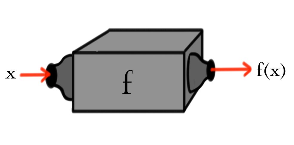
For part (a), the machine needed would look like the picture below.

$x$ $10x$.

This is just like a function $f(x)$ from calculus that takes in a number $x$ and spits out the number $f(x)=10x$. For part~($\ref{FVB}$), we need something more sophisticated.

$\begin{pmatrix}x\\ y\\ z\end{pmatrix}$ $\begin{pmatrix}z\\ -z\\ y-x\end{pmatrix}$.

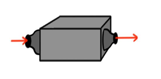
The inputs and outputs are both 3-vectors. You are probably getting the gist by now, but here is the machine needed for part~($\ref{FVC}$):

$p$$\begin{pmatrix}\int_{-1}^{1} p(y) dy\\ \int_{-1}^{1} y p(y) dy\end{pmatrix}$.

Here we input a polynomial and get a 2-vector as output!

By now you may be feeling overwhelmed and thinking that absolutely any function with any kind of vector as input and any other kind of vector as output can pop up next to strain your brain! Rest assured that linear algebra involves the study of only a very simple (yet very important) class of functions of vectors; its time to describe the essential characteristics of linear functions.

Let's use the letter $L$ for these functions and think again about vector addition and scalar multiplication. Lets suppose $v$ and $u$ are vectors and $c$ is a number. Then we already know that $u+v$ and $cu$ are also vectors. Since $L$ is a function of vectors, if we input $u$ into $L$, the output $L(u)$ will also be some sort of vector. The same goes for $L(v)$, $L(u+v)$ and $L(cu)$. Moreover, we can now also think about adding $L(u)$ and $L(v)$ to get yet another vector $L(u)+L(v)$ or of multiplying $L(u)$ by $c$ to obtain the vector $cL(u)$. Perhaps a picture of all this helps:

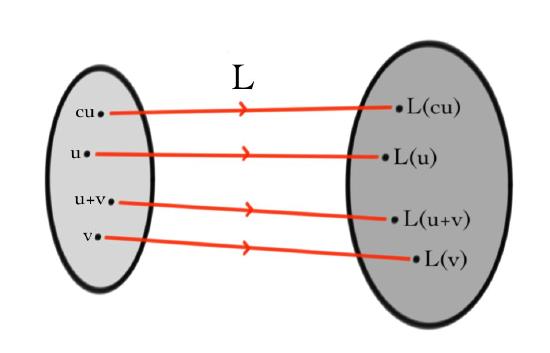
The ``blob'' on the left represents all the vectors that you are allowed to input into the function $L$, and the blob on the right denotes the corresponding outputs. Hopefully you noticed that there are two vectors apparently {\it not shown} on the blob of outputs:

\[ L(u)+L(v)\quad \&\quad cL(u)\, . $$

You might already be able to guess the values we would like these to take. If not, here's the answer, it's the key equation
of the whole class, from which everything else \hypertarget{twopart}{follows}:

1. Additivity:

$$L(u+v)=L(u)+L(v)\, .$$

2. Homogeneity:

$$L(cu)=cL(u)\, .$$

Most functions of vectors do not obey this requirement; linear algebra is the study of those that do. Notice that the additivity requirement says that the function $L$ respects vector addition: $\textit{it does not matter if you first add}$ $u$ $\textit{and}$ $v$ $\textit{and then input their sum into}$ $L$$\textit{, or first input}$ $u$ $\textit{and}$ $v$ $\textit{into}$ $L$ $\textit{separately and then add the outputs}$. The same holds for scalar multiplication--try writing out the scalar multiplication version of the italicized sentence. When a function of vectors obeys the additivity and homogeneity properties we say that it is $\textit{linear}$ (this is the "linear'' of linear algebra). Together, additivity and homogeneity are called $\textit{linearity}$. Other, equivalent, names for linear functions are:

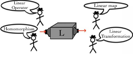
Function = Transformation = Operator

The questions in cases (a) - (d) of our example can all be restated as a single equation:

$$Lv = w$$

where $v$ is an unknown and $w$ a known vector, and $L$ is a linear transformation. To check that this is true, one needs to know the rules for adding vectors (both inputs and outputs) and then check linearity of $L$. Solving the equation $Lv=w$ often amounts to solving systems of linear equations, the skill you will learn in Chapter 2.

A great example is the derivative operator:

Example $\PageIndex{2}$: The derivative operator is linear

For any two functions $f(x)$, $g(x)$ and any number $c$, in calculus you probably learnt that the derivative operator satisfies

1. $\frac{d}{dx} (cf)=c\frac{d}{dx} f$,
2. $\frac{d}{dx}(f+g)=\frac{d}{dx}f+\frac{d}{dx}g$.

If we view functions as vectors with addition given by addition of functions and scalar multiplication just multiplication of functions by a constant, then these familiar properties of derivatives are just the linearity property of linear maps.

Before introducing matrices, notice that for linear maps $L$ we will often write simply $L u$ instead of $L(u)$. This is because the linearity property of a linear transformation $L$ means that $L(u)$ can be thought of as multiplying the vector $u$ by the linear operator $L$. For example, the linearity of $L$ implies that if $u,v$ are vectors and $c,d$ are numbers, then

$$L(c u + d v) = c L u + d L v,$$

which feels a lot like the regular rules of algebra for numbers. Notice though, that "$u L$'' makes no sense here.

Remark A sum of multiples of vectors $c u + dv$ is called a $\textit{linear combination}$ of $u$ and $v$.

Contributor

• David Cherney, Tom Denton, and Andrew Waldron (UC Davis)