
3.2: Graphical Solutions

( \newcommand{\kernel}{\mathrm{null}\,}\)
Before giving a more general algorithm for handling this problem and problems like it, we note that when the number of variables is small (preferably 2), a graphical technique can be used.
Inequalities, such as the four given in Pablo's problem, are often called constraints, and values of the variables that satisfy these constraints comprise the so-called feasible region. Since there are only two variables, this is easy to plot:
Example 3.2.1: Constraints and feasible region
Pablo's constraints are
x≥5y≥715≤x+y≤25.
Plotted in the (x,y) plane, this gives:
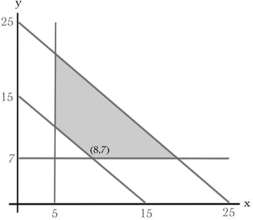
You might be able to see the solution to Pablo's problem already. Oranges are very sugary, so they should be kept low, thus y=7. Also, the less fruit the better, so the answer had better lie on the line x+y=15. Hence, the answer must be at the vertex (8,7). Actually this is a general feature of linear programming problems, the optimal answer must lie at a vertex of the feasible region. Rather than prove this, lets look at a plot of the linear function s(x,y)=5x+10y.
Example 3.2.2: The sugar function
Plotting the sugar function requires three dimensions:
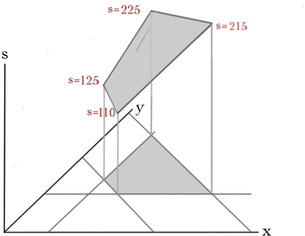
The plot of a linear function of two variables is a plane through the origin. Restricting the variables to the feasible region gives some lamina in 3-space. Since the function we want to optimize is linear (and assumedly non-zero), if we pick a point in the middle of this lamina, we can always increase/decrease the function by moving out to an edge and, in turn, along that edge to a corner. Applying this to the above picture, we see that Pablo's best option is 110 grams of sugar a week, in the form of 8 apples and 7 oranges.
It is worthwhile to contrast the optimization problem for a linear function with the non-linear case you may have seen in calculus courses:
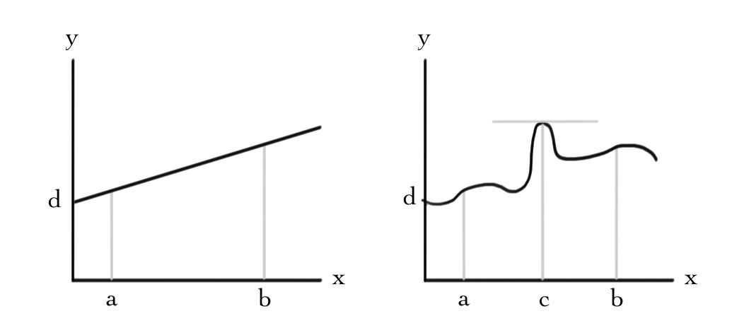
Here we have plotted the curve f(x)=d in the case where the function f is linear and non-linear. To optimize f in the interval [a,b], for the linear case we just need to compute and compare the values f(a) and f(b). In contrast, for non-linear functions it is necessary to also compute the derivative dfdx to study whether there are extrema inside the interval.
Contributor
David Cherney, Tom Denton, and Andrew Waldron (UC Davis)