
2.4E: Fitting Linear Models to Data (Exercises)
- Page ID
- 13900

section 2.4 exercise
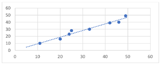
1. The following is data for the first and second quiz scores for 8 students in a class. Plot the points, then sketch a line that fits the data.
| First Quiz | 11 | 20 | 24 | 25 | 33 | 42 | 46 | 49 |
| Second Quiz | 10 | 16 | 23 | 28 | 30 | 39 | 40 | 49 |
2. Eight students were asked to estimate their score on a 10 point quiz. Their estimated and actual scores are given. Plot the points, then sketch a line that fits the data.
| Predicted | 5 | 7 | 6 | 8 | 10 | 9 | 10 | 7 |
| Actual | 6 | 6 | 7 | 8 | 9 | 9 | 10 | 6 |
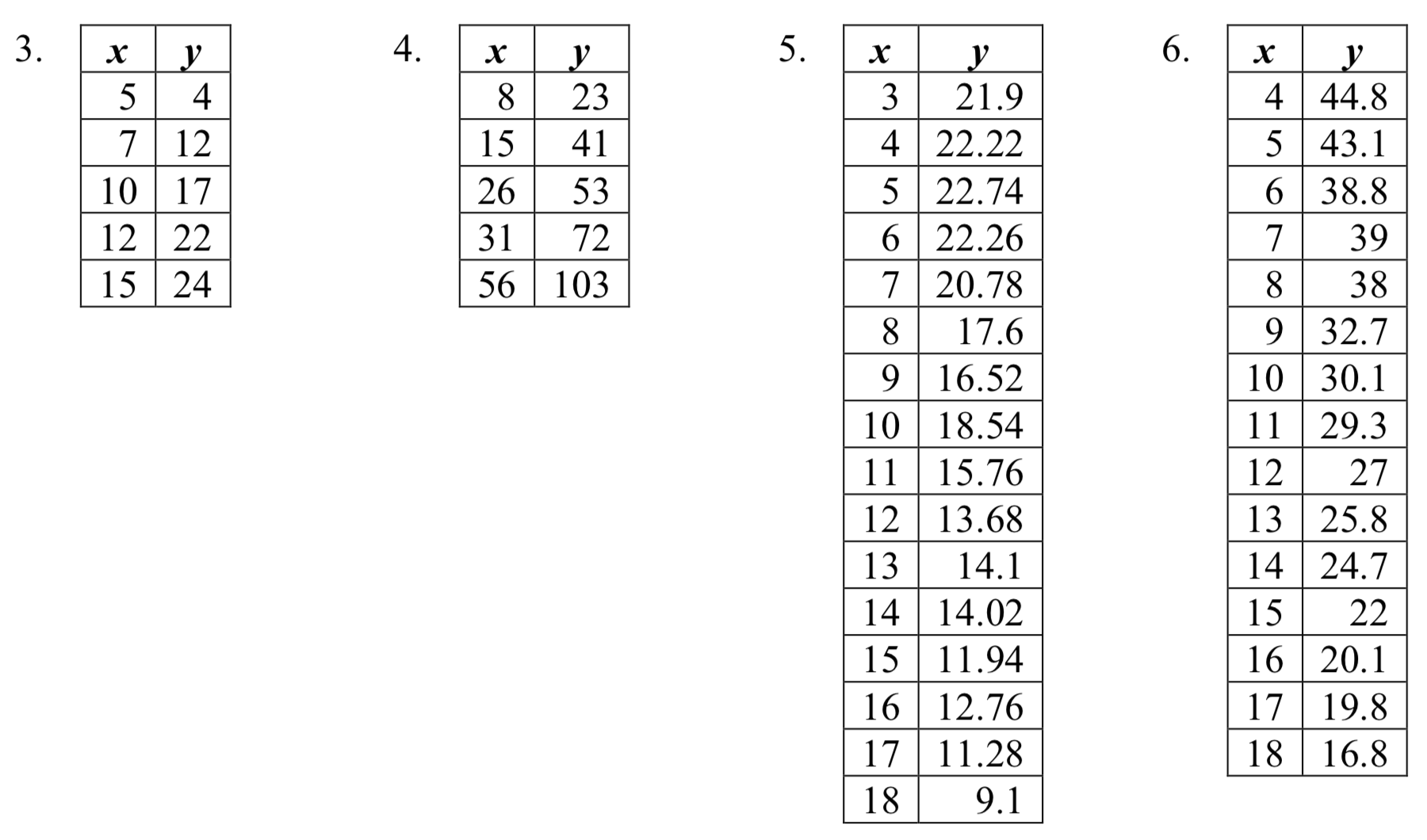
Based on each set of data given, calculate the regression line using your calculator or other technology tool, and determine the correlation coefficient.
7. A regression was run to determine if there is a relationship between hours of TV watched per day (\(x\)) and number of situps a person can do (\(y\)). The results of the regression are given below. Use this to predict the number of situps a person who watches 11 hours of TV can do.
\(y=ax+b\)
\(a=-1.341\)
\(b=32.234\)
\(r^2=0.803\)
\(r=-0.896\)
8. A regression was run to determine if there is a relationship between the diameter of a tree (\(x\), in inches) and the tree’s age (\(y\), in years). The results of the regression are given below. Use this to predict the age of a tree with diameter 10 inches.
\(y=ax+b\)
\(a=6.301\)
\(b=-1.044\)
\(r^2=0.940\)
\(r=0.970\)
Match each scatterplot shown below with one of the four specified correlations.
9. \(r = 0.95\) 10. \(r = -0.89\) 11. \(r = 0.26\) 12. \(r = -0.39\)
A 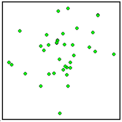 B
B 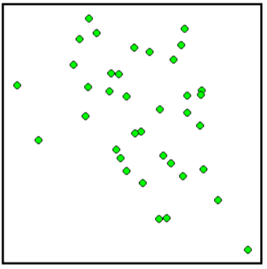 C
C 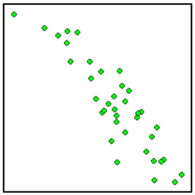 D
D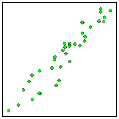
13. The US census tracks the percentage of persons 25 years or older who are college graduates. That data for several years is given below. Determine if the trend appears linear. If so and the trend continues, in what year will the percentage exceed 35%?
| Year | 1990 | 1992 | 1994 | 1996 | 1998 | 2000 | 2002 | 2004 | 2006 | 2008 |
| Percent Graduates | 21.3 | 21.4 | 22.2 | 23.6 | 24.4 | 25.6 | 26.7 | 27.7 | 28 | 29.4 |
14. The US import of wine (in hectoliters) for several years is given below. Determine if the trend appears linear. If so and the trend continues, in what year will imports exceed 12,000 hectoliters?
| Year | 1992 | 1994 | 1996 | 1998 | 2000 | 2002 | 2004 | 2006 | 2008 | 2009 |
| Imports | 2665 | 2688 | 3565 | 4129 | 4584 | 5655 | 6549 | 7950 | 8487 | 9462 |
- Answer
-
1.
3. \(y = 1.971x - 3.519\), \(r = 0.967\)
5. \(y = -0.901x + 26.04\), \(r = -0.968\)
7. \(17.483 \approx 17\ situps\)
9. D
11. A
13. Yes, trend appears linear because \(r = 0.994\) and will exceed 35% near the end of the year 2019.