1.3: Solving Triangles

Using information about some of the sides and angles of a triangle in order to find the unknown sides and angles is called "solving the triangle." If two sides of a triangle are known, the Pythagorean Theorem can be used to find the third side. If one of the acute angles in a right triangle is known, the other angle will be its complement with their sum being \(90^{\circ}\)

Suppose that we have a right triangle in which we know the sides, but no angles. Another situation could involve knowing the angles but just one side. How could we solve for the missing measurements in these situations?

Solving problems like these uses precalculated values of the trigonometric ratios to match the lengths with the appropriate angles and vice versa. Up until the 1980's, these values were printed in tables that were included in the back of every textbook (along with tables of logarithms), but have recently been programmed into calculators using methods that are studied in Calculus.

Most calculators have a button or function designed to find the inverse sine, inverse cosine and inverse tangent \(\left(\sin ^{-1}, \cos ^{-1}, \text {and } \tan ^{-1}\right),\) these are the functions that tell you the measure of the angle that has a sine, cosine or tangent equal to a particular value.
For example, if we are given an angle \(\theta\) and know that the \(\sin \theta=\frac{1}{2}\)

Then we can find \(\sin ^{-1}\left(\frac{1}{2}\right)\) on a calculator, which should return a value of \(30^{\circ} .\) If the calculator is in radian mode, it will return a value of \(\approx 0.523598776 .\) If you divided this number by \(\pi,\) you would get \(0.1 \overline{6},\) which means that \(0.523598776 \approx \frac{\pi}{6}\) In this chapter we will work mainly in degrees. In Chapter \(2,\) when we graph the trigonometric functions we will typically use radian measure.

Solve the triangle. Round side lengths to the nearest \(100^{t h}\) and angles to the nearest \(10^{\text {th }}\) of a degree.

We can find the third side of the triangle by using the Pythagorean Theorem.

\[ \begin{aligned}
a^{2}+5^{2} &=8^{2} \\
a^{2}+25 &=64
\end{aligned}
\] \(a^{2}=39\)
\[ a=\sqrt{39} \approx 6.24
\]

When solving problems of this type, I encourage people to use the most accurate values that are available in the problem. This way, there is less chance for rounding error to occur.

If we take the values for the sides that were given in the problem ( 5 and 8 ), then we can say that

\[ \begin{array}{c}
\cos \theta=\frac{5}{8} \\
\theta=\cos ^{-1}\left(\frac{5}{8}\right) \\
\theta \approx 51.3^{\circ}
\end{array}
\]

Then \(\alpha\) would be \(90^{\circ}-51.3^{\circ}=38.7^{\circ} \approx \alpha\)

Example 2
Solve the triangle. Round side lengths to the nearest \(100^{t h}\) and angles to the nearest \(10^{\text {th }}\) of a degree.

First, we can find the other angle in the right triangle: \(90^{\circ}-68^{\circ}=22^{\circ}\)
Next, to find the sides, we choose a trigonometric ratio for which we know one of the sides. In this problem, we can use either the sine or the cosine.
\(\sin 68^{\circ}=\frac{a}{5}\)
Approximating \(\sin 68^{\circ}\) on a calculator:
\(0.9272 \approx \frac{a}{5}\)
\[ 5 * 0.9272 \approx a
\] \(4.6 \approx a\)
When approximating a trigonometric value from the calculator, it is important to use at least 4 decimal places of accuracy. Again, this is to avoid rounding errors.
To solve for the remaining side we can either use the Pythagorean Theorem or use the method demonstrated above, but with the \(\cos 68^{\circ}\)

\(\cos 68^{\circ}=\frac{b}{5}\)
Approximating cos \(68^{\circ}\) on a calculator:
\[ \begin{array}{c}
0.3746 \approx \frac{b}{5} \\
5 * 0.3746 \approx b \\
1.9 \approx b
\end{array}
\] If we use the Pythagorean Theorem with two sides of the triangle to find the third, then we would say that:
\[ \begin{array}{c}
b^{2}+4.6^{2}=5^{2} \\
b^{2}+21.16=25 \\
b^{2}=3.84 \\
b=\sqrt{3.84} \approx 1.959 \approx 2.0
\end{array}
\] The rounding error in this example comes from the fact that the first side we found was not exactly \(4.6 .\) If we wanted a more accurate answer that matches the answer we found using the cosine ratio, we just need more accuracy in the leg of the triangle we found.
Calculating \(5 * \sin 68^{\circ} \approx 4.636\) should provide enough accuracy.
\[ \begin{array}{c}
b^{2}+4.636^{2}=5^{2} \\
b^{2}+21.492496=25 \\
b^{2}=3.507504 \\
b=\sqrt{3.507504} \approx 1.8728 \approx 1.9
\end{array}
\]

Example 3
Solve the triangle. Round side lengths to the nearest \(100^{t h}\) and angles to the nearest \(10^{\text {th }}\) of a degree.

If we convert the angle \(22^{\circ} 10^{\prime}\) to \(22.1 \overline{6}^{\circ},\) then the other acute angle in the right triangle is \(90^{\circ}-22.1 \overline{6}^{\circ}=67.8 \overline{3}^{\circ}\) or \(67^{\circ} 50^{\prime}\)
Finding the remaining sides requires the use of either the cosine or tangent function.
\[ \cos 22.1 \overrightarrow{6}^{\circ}=\frac{40}{c}
\] Approximating cos \(22.1 \overline{6}^{\circ}\) on a calculator:
\[ 0.9261 \approx \frac{40}{c}
\] Next we need to multiply on both sides by \(c:\)
\[ c * 0.9261 \approx \frac{40}{c} * c
\] \(0.9261 c \approx 40\)
Then divide on both sides by 0.9261:
\[ \begin{array}{c}
\frac{0.9261 c}{0.9261} \approx \frac{40}{0.9261} \\
c \approx 43.2
\end{array}
\]

To find the other leg of the triangle, we can use the tangent ratio.
\[ \tan 22.1 \overline{6}^{\circ}=\frac{a}{40}
\] Approximating tan \(22.1 \overline{6}^{\circ}\) on a calculator:
\[ 0.4074 \approx \frac{a}{40}
\] Then, multiply on both sides by 40:
\[ \begin{array}{c}
40 * 0.4074 \approx a \\
16.3 \approx a
\end{array}
\] We can check this answer by the Pythagorean Theorem:
\[ 16.3^{2}+40^{2}=1865.69
\] \[ \sqrt{1865.69} \approx 43.2
\]

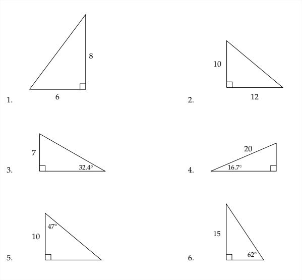
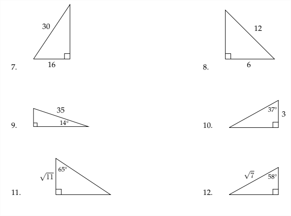
Exercises 1.3
In each problem below, solve the triangle. Round side lengths to the nearest \(100^{t h}\) and angle measures to the nearest \(10^{\text {th }}\) of a degree.