3.3: Trigonometric Equations
- Page ID
- 37221
\( \newcommand{\vecs}[1]{\overset { \scriptstyle \rightharpoonup} {\mathbf{#1}} } \)
\( \newcommand{\vecd}[1]{\overset{-\!-\!\rightharpoonup}{\vphantom{a}\smash {#1}}} \)
\( \newcommand{\dsum}{\displaystyle\sum\limits} \)
\( \newcommand{\dint}{\displaystyle\int\limits} \)
\( \newcommand{\dlim}{\displaystyle\lim\limits} \)
\( \newcommand{\id}{\mathrm{id}}\) \( \newcommand{\Span}{\mathrm{span}}\)
( \newcommand{\kernel}{\mathrm{null}\,}\) \( \newcommand{\range}{\mathrm{range}\,}\)
\( \newcommand{\RealPart}{\mathrm{Re}}\) \( \newcommand{\ImaginaryPart}{\mathrm{Im}}\)
\( \newcommand{\Argument}{\mathrm{Arg}}\) \( \newcommand{\norm}[1]{\| #1 \|}\)
\( \newcommand{\inner}[2]{\langle #1, #2 \rangle}\)
\( \newcommand{\Span}{\mathrm{span}}\)
\( \newcommand{\id}{\mathrm{id}}\)
\( \newcommand{\Span}{\mathrm{span}}\)
\( \newcommand{\kernel}{\mathrm{null}\,}\)
\( \newcommand{\range}{\mathrm{range}\,}\)
\( \newcommand{\RealPart}{\mathrm{Re}}\)
\( \newcommand{\ImaginaryPart}{\mathrm{Im}}\)
\( \newcommand{\Argument}{\mathrm{Arg}}\)
\( \newcommand{\norm}[1]{\| #1 \|}\)
\( \newcommand{\inner}[2]{\langle #1, #2 \rangle}\)
\( \newcommand{\Span}{\mathrm{span}}\) \( \newcommand{\AA}{\unicode[.8,0]{x212B}}\)
\( \newcommand{\vectorA}[1]{\vec{#1}} % arrow\)
\( \newcommand{\vectorAt}[1]{\vec{\text{#1}}} % arrow\)
\( \newcommand{\vectorB}[1]{\overset { \scriptstyle \rightharpoonup} {\mathbf{#1}} } \)
\( \newcommand{\vectorC}[1]{\textbf{#1}} \)
\( \newcommand{\vectorD}[1]{\overrightarrow{#1}} \)
\( \newcommand{\vectorDt}[1]{\overrightarrow{\text{#1}}} \)
\( \newcommand{\vectE}[1]{\overset{-\!-\!\rightharpoonup}{\vphantom{a}\smash{\mathbf {#1}}}} \)
\( \newcommand{\vecs}[1]{\overset { \scriptstyle \rightharpoonup} {\mathbf{#1}} } \)
\(\newcommand{\longvect}{\overrightarrow}\)
\( \newcommand{\vecd}[1]{\overset{-\!-\!\rightharpoonup}{\vphantom{a}\smash {#1}}} \)
\(\newcommand{\avec}{\mathbf a}\) \(\newcommand{\bvec}{\mathbf b}\) \(\newcommand{\cvec}{\mathbf c}\) \(\newcommand{\dvec}{\mathbf d}\) \(\newcommand{\dtil}{\widetilde{\mathbf d}}\) \(\newcommand{\evec}{\mathbf e}\) \(\newcommand{\fvec}{\mathbf f}\) \(\newcommand{\nvec}{\mathbf n}\) \(\newcommand{\pvec}{\mathbf p}\) \(\newcommand{\qvec}{\mathbf q}\) \(\newcommand{\svec}{\mathbf s}\) \(\newcommand{\tvec}{\mathbf t}\) \(\newcommand{\uvec}{\mathbf u}\) \(\newcommand{\vvec}{\mathbf v}\) \(\newcommand{\wvec}{\mathbf w}\) \(\newcommand{\xvec}{\mathbf x}\) \(\newcommand{\yvec}{\mathbf y}\) \(\newcommand{\zvec}{\mathbf z}\) \(\newcommand{\rvec}{\mathbf r}\) \(\newcommand{\mvec}{\mathbf m}\) \(\newcommand{\zerovec}{\mathbf 0}\) \(\newcommand{\onevec}{\mathbf 1}\) \(\newcommand{\real}{\mathbb R}\) \(\newcommand{\twovec}[2]{\left[\begin{array}{r}#1 \\ #2 \end{array}\right]}\) \(\newcommand{\ctwovec}[2]{\left[\begin{array}{c}#1 \\ #2 \end{array}\right]}\) \(\newcommand{\threevec}[3]{\left[\begin{array}{r}#1 \\ #2 \\ #3 \end{array}\right]}\) \(\newcommand{\cthreevec}[3]{\left[\begin{array}{c}#1 \\ #2 \\ #3 \end{array}\right]}\) \(\newcommand{\fourvec}[4]{\left[\begin{array}{r}#1 \\ #2 \\ #3 \\ #4 \end{array}\right]}\) \(\newcommand{\cfourvec}[4]{\left[\begin{array}{c}#1 \\ #2 \\ #3 \\ #4 \end{array}\right]}\) \(\newcommand{\fivevec}[5]{\left[\begin{array}{r}#1 \\ #2 \\ #3 \\ #4 \\ #5 \\ \end{array}\right]}\) \(\newcommand{\cfivevec}[5]{\left[\begin{array}{c}#1 \\ #2 \\ #3 \\ #4 \\ #5 \\ \end{array}\right]}\) \(\newcommand{\mattwo}[4]{\left[\begin{array}{rr}#1 \amp #2 \\ #3 \amp #4 \\ \end{array}\right]}\) \(\newcommand{\laspan}[1]{\text{Span}\{#1\}}\) \(\newcommand{\bcal}{\cal B}\) \(\newcommand{\ccal}{\cal C}\) \(\newcommand{\scal}{\cal S}\) \(\newcommand{\wcal}{\cal W}\) \(\newcommand{\ecal}{\cal E}\) \(\newcommand{\coords}[2]{\left\{#1\right\}_{#2}}\) \(\newcommand{\gray}[1]{\color{gray}{#1}}\) \(\newcommand{\lgray}[1]{\color{lightgray}{#1}}\) \(\newcommand{\rank}{\operatorname{rank}}\) \(\newcommand{\row}{\text{Row}}\) \(\newcommand{\col}{\text{Col}}\) \(\renewcommand{\row}{\text{Row}}\) \(\newcommand{\nul}{\text{Nul}}\) \(\newcommand{\var}{\text{Var}}\) \(\newcommand{\corr}{\text{corr}}\) \(\newcommand{\len}[1]{\left|#1\right|}\) \(\newcommand{\bbar}{\overline{\bvec}}\) \(\newcommand{\bhat}{\widehat{\bvec}}\) \(\newcommand{\bperp}{\bvec^\perp}\) \(\newcommand{\xhat}{\widehat{\xvec}}\) \(\newcommand{\vhat}{\widehat{\vvec}}\) \(\newcommand{\uhat}{\widehat{\uvec}}\) \(\newcommand{\what}{\widehat{\wvec}}\) \(\newcommand{\Sighat}{\widehat{\Sigma}}\) \(\newcommand{\lt}{<}\) \(\newcommand{\gt}{>}\) \(\newcommand{\amp}{&}\) \(\definecolor{fillinmathshade}{gray}{0.9}\)In the previous section on trigonometric identities we worked with equations that would be true for all values of a particular angle \(\theta .\) These are sort of like the algebraic equations whose solution set is "all real numbers," like \(2 x+10=\) \(2(x+1)+8 .\) In this section, we will solve trigonometric equations whose solution set involves only certain values for the angle in question. Because of the cyclical nature of the angles we're working with, there will often be an infinite number of solutions although not "all real numbers."
Example 1
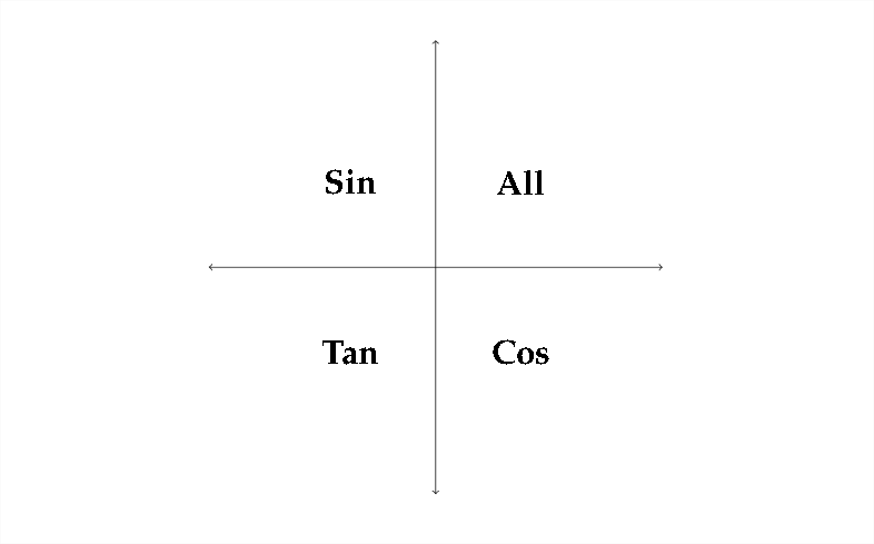
Here's an example. Suppose that we consider the equation \(\sin x=0.5 .\) Whether we use technology, a table or reasoning to solve this equation, it's clear that one solution is \(30^{\circ} .\) However, remember from the beginning of Chapter 2 that the sine function is positive in Quadrant \(\Pi\). That means that a second quadrant angle with a reference angle of \(30^{\circ}\) also has a sine equal to \(0.5 .\) Recall the ASTC diagram from Chapter 2 :

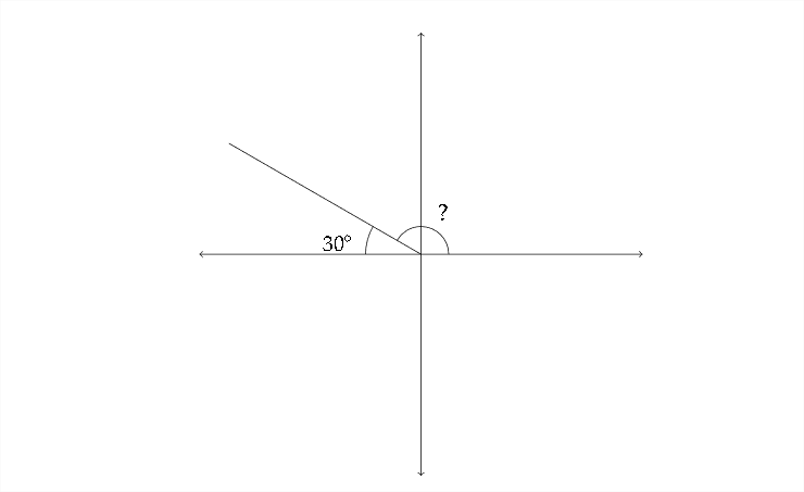
So, the sine function is positive in Quadrants I and \(\Pi\). This means that in addition to a solution of \(30^{\circ},\) there is another solution in Quadrant \(\Pi\). As mentioned above, this second quadrant solution has a reference angle of \(30^{\circ}\)

To find this angle, we simply subtract \(180^{\circ}-30^{\circ}=150^{\circ}\)
In Quadrant \(\Pi,\) we subtract the reference angle from \(180^{\circ}\)
In Quadrant \(\Pi\), we add the reference angle to \(180^{\circ}\)
In Quadrant \(\Pi V\), we subtract the reference angle from \(360^{\circ}\)
So, the solutions to the equation \(\sin x=0.5\) between \(0^{\circ}\) and \(360^{\circ}\) are \(x=30^{\circ}, 150^{\circ}\) In this chapter we will consider mainly solutions with this restriction:
\[
0^{\circ} \leq x<360^{\circ}
\]
The infinite solutions to this equation can be expressed as:
\[
30^{\circ}+n \cdot 360^{\circ} \text { and } 150^{\circ}+n \cdot 360^{\circ}
\]
Let's look at another example:
Example 2
Find all solutions of the given equation for \(0^{\circ} \leq x<360^{\circ}\)
\(\tan x=4\)
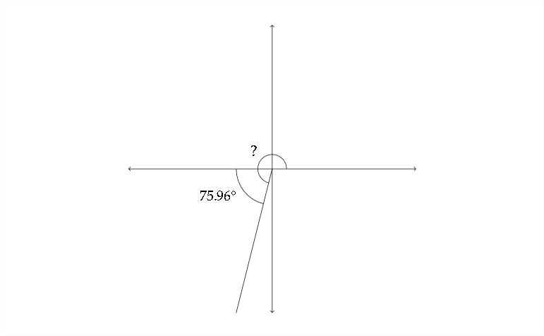
Using a calculator to find \(\tan ^{-1}(4),\) we find that it returns an answer of \(x \approx 75.96^{\circ}\) So this is the solution to the equation that lies in QuadrantI. The tangent function is also positive in Quadrant \(\Pi\), so we should also consider the third quadrant angle with a reference angle of \(75.96^{\circ}\)

In Quadrant \(\Pi\), we add the reference angle to \(180^{\circ}\)
\(180^{\circ}+75.96^{\circ}=255.96^{\circ},\) so our solutions for this equation are \(x \approx 75.96^{\circ}, 255.96^{\circ}\)
Often, calculators are programmed to return an angle value that is not between \(0^{\circ} \leq x<360^{\circ}\)
Example 3
Find all solutions of the given equation for \(0^{\circ} \leq x<360^{\circ}\)
\(\sin x=-0.25\)
Solving this on a TI calculator would generally return a value of \(-14.5^{\circ} .\) However, \(-14.5^{\circ}\) is clearly not between \(0^{\circ}\) and \(360^{\circ}\), so we need to use this information to find the solutions that are between \(0^{\circ}\) and \(360^{\circ}\)
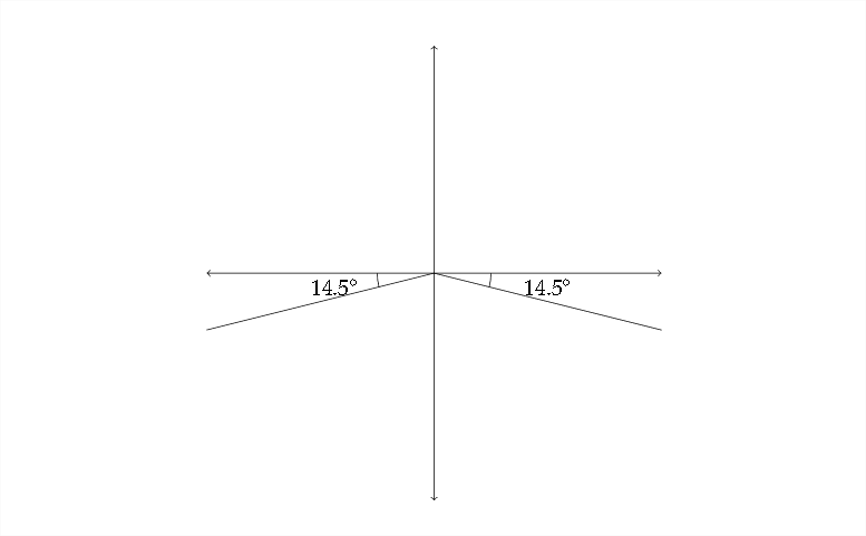
With the calculator returning a vlue of \(-14.5^{\circ},\) we know that the reference angle for all answers will be \(14.5^{\circ} .\) Knowing this, we can say that the sine is negative in Quadrants III and IV, so we'll need angles in those quadrants with reference angles of \(14.5^{\circ}\)

In Quadrant \(\Pi\) we'll add \(180^{\circ}\) to the reference angle: \(180^{\circ}+14.5^{\circ}=194.5^{\circ}\)
In Quadrant \(\Pi\) we'll subtract the reference angle from \(360^{\circ}: 360^{\circ}-14.5^{\circ}=345.5^{\circ}\)
So, \(x \approx 194.5^{\circ}, 345.5^{\circ}\)
Some trigonometric equations have no real number solutions. The equation \(\sin x=2\) has no real number solutions. Recall that the sine ratio was originally defined as the ratio of the side opposite an angle to the hypotenuse. The hypotenuse is always the longest side in a right triangle so there is no way the sine function could be greater than 1 if we're working with real-valued angles. However, in the same way that complex numbers are used to solve equations like \(x^{2}=-7,\) complex-valued angles can be used to solve equations such as \(\sin x=2\) We won't go into this here, however, there is a relatively straightforward way to solve these equations.
If you encounter an equation like \(\cos x=3\) and are solving for values of \(x\) \(0^{\circ} \leq x<360^{\circ},\) then the proper response is "no solution" or "no real solution." However, remember that the tangent function can take any value between \(-\infty\) and \(\infty\)
Example 4
Solving an equation that includes a reciprocal trigonometric function simply involves the extra step of finding the reciprocal:
Find all solutions of the given equation for \(0^{\circ} \leq x<360^{\circ}\)
\(\sec x=12\)
The trick here is to restate the equation so that we can use the preprogrammed values from a calculator to find the solution.
If \(\sec x=12\) then \(\cos x=\frac{1}{12} .\) Finding \(\cos ^{-1}\left(\frac{1}{12}\right)\) gives a solution of \(x \approx 85.2^{\circ}\)
The cosine and the secant are both positive in Quadrant \(\Pi \mathrm{V}\), so we'll also want a fourth quadrant angle whose reference angle is \(85.2^{\circ}\)

In Quadrant \(\Pi\), we'll subtract the reference angle from \(360^{\circ}\)
\[
\begin{array}{c}
360^{\circ}-85.2^{\circ} \approx 274.8^{\circ} \\
x \approx 85.2^{\circ}, 274.8^{\circ}
\end{array}
\]
Example 5
Solving a quadratic trigonometric equation often involves the use of the quadratic formula:
Find all solutions of the given equation for \(0^{\circ} \leq x<360^{\circ}\)
\(2 \sin ^{2} x-\sin x-2=0\)
Using the quadratic formula we arrive at approximate values for \(\sin x\) of \(\sin x \approx-0.7808,1.2808\)
The solution \(\sin x \approx 1.2808\) yields no real solutions, so we will focus on solving \(\sin x \approx-0.7808\)
Finding \(\sin ^{-1}(-0.7808)\) gives us an answer of \(\approx-51.3^{\circ} .\) This means our answers will lie in Quadrants III and IV with reference angles of \(51.3^{\circ} .\) In Quadrant III we'll say \(180^{\circ}+51.3^{\circ} \approx 231.3^{\circ} .\) In Quadrant \(\mathrm{IV}\), we'll subtract the reference angle from \(360^{\circ}: 360^{\circ}-51.3^{\circ} \approx 308.7^{\circ}\)
\(\mathrm{So}, x \approx 231.3^{\circ}, 308.7^{\circ}\)
Exercises 3.3
Find all solutions for \(0^{\circ} \leq x<360^{\circ}\) Round all angle measures to the nearest \(10^{\text {th }}\) of a degree.
1. \(\cos x-0.75=0\)
2. \(\sin x+0.432=0\)
3. \( 3 \sin x-5=0\)
4. \(\sin x-4=0\)
5. \( 3 \sec x+8=0\)
6. \( 4 \csc x+9=0\)
7. \( 3-5 \sin x=4 \sin x+1\)
8. \( 4 \cos x-5=\cos x-3\)
9. \( 3 \tan ^{2} x+2 \tan x=0\)
10. \( 4 \cos ^{2} x-\cos x=0\)
11. \( 3 \cos ^{2} x+5 \cos x-2=0\)
12. \( 2 \cot ^{2} x-7 \cot x+3=0\)
13. \( 2 \tan ^{2} x-\tan x-10=0\)
14. \( 2 \sin ^{2} x+5 \sin x+3=0\)
15. \( 2 \cos ^{2} x-5 \cos x-5=0\)
16. \( 3 \sin ^{2} x-\sin x-1=0\)


