1.5: Rotations and Reflections of Angles
- Page ID
- 3248
\( \newcommand{\vecs}[1]{\overset { \scriptstyle \rightharpoonup} {\mathbf{#1}} } \)
\( \newcommand{\vecd}[1]{\overset{-\!-\!\rightharpoonup}{\vphantom{a}\smash {#1}}} \)
\( \newcommand{\id}{\mathrm{id}}\) \( \newcommand{\Span}{\mathrm{span}}\)
( \newcommand{\kernel}{\mathrm{null}\,}\) \( \newcommand{\range}{\mathrm{range}\,}\)
\( \newcommand{\RealPart}{\mathrm{Re}}\) \( \newcommand{\ImaginaryPart}{\mathrm{Im}}\)
\( \newcommand{\Argument}{\mathrm{Arg}}\) \( \newcommand{\norm}[1]{\| #1 \|}\)
\( \newcommand{\inner}[2]{\langle #1, #2 \rangle}\)
\( \newcommand{\Span}{\mathrm{span}}\)
\( \newcommand{\id}{\mathrm{id}}\)
\( \newcommand{\Span}{\mathrm{span}}\)
\( \newcommand{\kernel}{\mathrm{null}\,}\)
\( \newcommand{\range}{\mathrm{range}\,}\)
\( \newcommand{\RealPart}{\mathrm{Re}}\)
\( \newcommand{\ImaginaryPart}{\mathrm{Im}}\)
\( \newcommand{\Argument}{\mathrm{Arg}}\)
\( \newcommand{\norm}[1]{\| #1 \|}\)
\( \newcommand{\inner}[2]{\langle #1, #2 \rangle}\)
\( \newcommand{\Span}{\mathrm{span}}\) \( \newcommand{\AA}{\unicode[.8,0]{x212B}}\)
\( \newcommand{\vectorA}[1]{\vec{#1}} % arrow\)
\( \newcommand{\vectorAt}[1]{\vec{\text{#1}}} % arrow\)
\( \newcommand{\vectorB}[1]{\overset { \scriptstyle \rightharpoonup} {\mathbf{#1}} } \)
\( \newcommand{\vectorC}[1]{\textbf{#1}} \)
\( \newcommand{\vectorD}[1]{\overrightarrow{#1}} \)
\( \newcommand{\vectorDt}[1]{\overrightarrow{\text{#1}}} \)
\( \newcommand{\vectE}[1]{\overset{-\!-\!\rightharpoonup}{\vphantom{a}\smash{\mathbf {#1}}}} \)
\( \newcommand{\vecs}[1]{\overset { \scriptstyle \rightharpoonup} {\mathbf{#1}} } \)
\( \newcommand{\vecd}[1]{\overset{-\!-\!\rightharpoonup}{\vphantom{a}\smash {#1}}} \)
\(\newcommand{\avec}{\mathbf a}\) \(\newcommand{\bvec}{\mathbf b}\) \(\newcommand{\cvec}{\mathbf c}\) \(\newcommand{\dvec}{\mathbf d}\) \(\newcommand{\dtil}{\widetilde{\mathbf d}}\) \(\newcommand{\evec}{\mathbf e}\) \(\newcommand{\fvec}{\mathbf f}\) \(\newcommand{\nvec}{\mathbf n}\) \(\newcommand{\pvec}{\mathbf p}\) \(\newcommand{\qvec}{\mathbf q}\) \(\newcommand{\svec}{\mathbf s}\) \(\newcommand{\tvec}{\mathbf t}\) \(\newcommand{\uvec}{\mathbf u}\) \(\newcommand{\vvec}{\mathbf v}\) \(\newcommand{\wvec}{\mathbf w}\) \(\newcommand{\xvec}{\mathbf x}\) \(\newcommand{\yvec}{\mathbf y}\) \(\newcommand{\zvec}{\mathbf z}\) \(\newcommand{\rvec}{\mathbf r}\) \(\newcommand{\mvec}{\mathbf m}\) \(\newcommand{\zerovec}{\mathbf 0}\) \(\newcommand{\onevec}{\mathbf 1}\) \(\newcommand{\real}{\mathbb R}\) \(\newcommand{\twovec}[2]{\left[\begin{array}{r}#1 \\ #2 \end{array}\right]}\) \(\newcommand{\ctwovec}[2]{\left[\begin{array}{c}#1 \\ #2 \end{array}\right]}\) \(\newcommand{\threevec}[3]{\left[\begin{array}{r}#1 \\ #2 \\ #3 \end{array}\right]}\) \(\newcommand{\cthreevec}[3]{\left[\begin{array}{c}#1 \\ #2 \\ #3 \end{array}\right]}\) \(\newcommand{\fourvec}[4]{\left[\begin{array}{r}#1 \\ #2 \\ #3 \\ #4 \end{array}\right]}\) \(\newcommand{\cfourvec}[4]{\left[\begin{array}{c}#1 \\ #2 \\ #3 \\ #4 \end{array}\right]}\) \(\newcommand{\fivevec}[5]{\left[\begin{array}{r}#1 \\ #2 \\ #3 \\ #4 \\ #5 \\ \end{array}\right]}\) \(\newcommand{\cfivevec}[5]{\left[\begin{array}{c}#1 \\ #2 \\ #3 \\ #4 \\ #5 \\ \end{array}\right]}\) \(\newcommand{\mattwo}[4]{\left[\begin{array}{rr}#1 \amp #2 \\ #3 \amp #4 \\ \end{array}\right]}\) \(\newcommand{\laspan}[1]{\text{Span}\{#1\}}\) \(\newcommand{\bcal}{\cal B}\) \(\newcommand{\ccal}{\cal C}\) \(\newcommand{\scal}{\cal S}\) \(\newcommand{\wcal}{\cal W}\) \(\newcommand{\ecal}{\cal E}\) \(\newcommand{\coords}[2]{\left\{#1\right\}_{#2}}\) \(\newcommand{\gray}[1]{\color{gray}{#1}}\) \(\newcommand{\lgray}[1]{\color{lightgray}{#1}}\) \(\newcommand{\rank}{\operatorname{rank}}\) \(\newcommand{\row}{\text{Row}}\) \(\newcommand{\col}{\text{Col}}\) \(\renewcommand{\row}{\text{Row}}\) \(\newcommand{\nul}{\text{Nul}}\) \(\newcommand{\var}{\text{Var}}\) \(\newcommand{\corr}{\text{corr}}\) \(\newcommand{\len}[1]{\left|#1\right|}\) \(\newcommand{\bbar}{\overline{\bvec}}\) \(\newcommand{\bhat}{\widehat{\bvec}}\) \(\newcommand{\bperp}{\bvec^\perp}\) \(\newcommand{\xhat}{\widehat{\xvec}}\) \(\newcommand{\vhat}{\widehat{\vvec}}\) \(\newcommand{\uhat}{\widehat{\uvec}}\) \(\newcommand{\what}{\widehat{\wvec}}\) \(\newcommand{\Sighat}{\widehat{\Sigma}}\) \(\newcommand{\lt}{<}\) \(\newcommand{\gt}{>}\) \(\newcommand{\amp}{&}\) \(\definecolor{fillinmathshade}{gray}{0.9}\)Now that we know how to deal with angles of any measure, we will take a look at how certain geometric operations can help simplify the use of trigonometric functions of any angle, and how some basic relations between those functions can be made. The two operations on which we will concentrate in this section are rotation and reflection.
To rotate an angle means to rotate its terminal side around the origin when the angle is in standard position. For example, suppose we rotate an angle \(\theta \) around the origin by \(90^\circ \) in the counterclockwise direction. In Figure 1.5.1 we see an angle \(\theta \) in QI which is rotated by \(90^\circ \), resulting in the angle \(\theta + 90^\circ \) in QII. Notice that the complement of \(\theta \) in the right triangle in QI is the same as the supplement of the angle \(\theta + 90^\circ \) in QII, since the sum of \(\theta \), its complement, and \(90^\circ \) equals \(180^\circ \). This forces the other angle of the right triangle in QII to be \(\theta \).
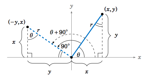
Thus, the right triangle in QI is similar to the right triangle in QII, since the triangles have the same angles. The rotation of \(\theta \) by \(90^\circ \) does not change the length \(r \) of its terminal side, so the hypotenuses of the similar right triangles are equal, and hence by similarity the remaining corresponding sides are also equal. Using Figure 1.5.1 to match up those corresponding sides shows that the point \((-y,x) \) is on the terminal side of \(\theta + 90^\circ\) when \((x,y) \) is on the terminal side of \(\theta \). Hence, by definition,
\[\nonumber \sin\;(\theta + 90^\circ) ~ = ~ \frac{x}{r} ~=~ \cos\;\theta ~,~~
\cos\;(\theta + 90^\circ) ~ = ~ \frac{-y}{r} ~=~ -\sin\;\theta ~,~~
\tan\;(\theta + 90^\circ) ~ = ~ \frac{x}{-y} ~=~ -\cot\;\theta ~. \nonumber \]
Though we showed this for \(\theta \) in QI, it is easy (see Exercise 4) to use similar arguments for the other quadrants. In general, the following relations hold for all angles \(\theta\):
\[\sin\;(\theta + 90^\circ) ~ = ~ \cos\;\theta \label{1.4} \]
\[ \cos\;(\theta + 90^\circ) ~ = ~ -\sin\;\theta \label{1.5} \]
\[ \tan\;(\theta + 90^\circ) ~ = ~ -\cot\;\theta \label{1.6} \]
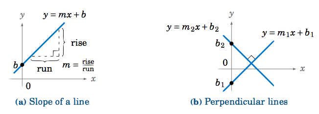
Recall that any nonvertical line in the \(xy\)-coordinate plane can be written as \(y=mx+b \), where \(m \) is the slope of the line (defined as \(m = \frac{\text{rise}}{\text{run}} \) ) and \(b \) is the \(y\)-intercept}, i.e. where the line crosses the \(y\)-axis (see Figure 1.5.2(a)). We will show that the slopes of perpendicular lines are negative reciprocals. That is, if \(y=m_{1}x+b_1 \) and \(y=m_{2}x+b_2 \) are nonvertical and nonhorizontal perpendicular lines, then \(m_2 = -\frac{1}{m_1} \) (see Figure 1.5.2(b)).
First, suppose that a line \(y=mx+b \) has nonzero slope. The line crosses the \(x\)-axis somewhere, so let \(\theta \) be the angle that the positive \(x\)-axis makes with the part of the line above the \(x\)-axis, as in Figure 1.5.3. For \(m > 0 \) we see that \(\theta \) is acute and \(\tan\;\theta = \frac{\text{rise}}{\text{run}} = m \).
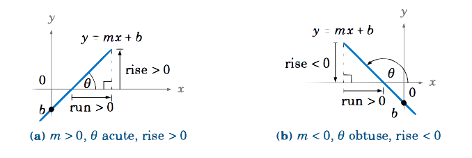
If \(m < 0 \), then we see that \(\theta \) is obtuse and the rise is negative. Since the run is always positive, our definition of \(\tan\;\theta \) from Section 1.4 means that \(\tan\;\theta = \frac{-\text{rise}}{-\text{run}} = \frac{\text{rise}}{\text{run}} = m \) (just imagine in Figure 1.5.3(b) the entire line being shifted horizontally to go through the origin, so that \(\theta \) is unchanged and the point \((-\text{run},-\text{rise}) \) is on the terminal side of \(\theta\)). Hence:
For a line \(y=mx+b \) with \(m \ne 0 \), the slope is given by \(m = \tan\;\theta\, \), where \(\theta \) is the angle formed by the positive \(x\)-axis and the part of the line above the \(x\)-axis.}
Now, in Figure 1.5.2(b) we see that if two lines \(y=m_{1}x+b_1 \) and \(y=m_{2}x+b_2 \) are perpendicular then rotating one line counterclockwise by \(90^\circ \) around the point of intersection gives us the second line. So if \(\theta \) is the angle that the line \(y=m_{1}x+b_1 \) makes with the positive \(x\)-axis, then \(\theta + 90^\circ \) is the angle that the line \(y=m_{2}x+b_2 \) makes with the positive \(x\)-axis. So by what we just showed, \(m_1 = \tan\;\theta \) and \(m_2 = \tan\;(\theta + 90^\circ) \). But by formula Equation \ref{1.6} we know that \(\tan\;(\theta + 90^\circ) = -\cot\;\theta \). Hence, \(m_2 = -\cot\;\theta = -\frac{1}{\tan\;\theta} = -\frac{1}{m_1} \). \(\textbf{QED}\)
Rotating an angle \(\theta \) by \(90^\circ \) in the clockwise direction results in the angle \(\theta - 90^\circ \). We could use another geometric argument to derive trigonometric relations involving \(\theta - 90^\circ \), but it is easier to use a simple trick: since Equations \ref{1.4}-\ref{1.6} hold for any angle \(\theta \), just replace \(\theta \) by \(\theta - 90^\circ \) in each formula. Since \((\theta - 90^\circ) + 90^\circ = \theta \), this gives us:
\[\label{1.7} \sin\;(\theta - 90^\circ) ~ = ~ -\cos\;\theta \]
\[\label{1.8} \cos\;(\theta - 90^\circ) ~ = ~ \sin\;\theta \]
\[\label{1.9}\tan\;(\theta - 90^\circ) ~ = ~ -\cot\;\theta \]
We now consider rotating an angle \(\theta \) by \(180^\circ \). Notice from Figure 1.5.4 that the angles \(\theta \pm 180^\circ \) have the same terminal side, and are in the quadrant opposite \(\theta \).

Since \((-x,-y) \) is on the terminal side of \(\theta \pm 180^\circ \) when \((x,y) \) is on the terminal side of \(\theta \), we get the following relations, which hold for all \(\theta\):
\[\label{1.10}\sin\;(\theta \pm 180^\circ) ~ = ~ -\sin\;\theta \]
\[\label{1.11} \cos\;(\theta \pm 180^\circ) ~ = ~ -\cos\;\theta \]
\[\label{1.12}\tan\;(\theta \pm 180^\circ) ~ = ~ \tan\;\theta \]
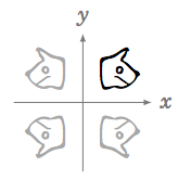
A reflection is simply the mirror image of an object. For example, in Figure 1.5.5 the original object is in QI, its reflection around the \(y\)-axis is in QII, and its reflection around the \(x\)-axis is in QIV. Notice that if we first reflect the object in QI around the \(y\)-axis and then follow that with a reflection around the \(x\)-axis, we get an image in QIII. That image is the reflection around the origin of the original object, and it is equivalent to a rotation of \(180^\circ \) around the origin. Notice also that a reflection around the \(y\)-axis is equivalent to a reflection around the \(x\)-axis followed by a rotation of \(180^\circ \) around the origin.
Applying this to angles, we see that the reflection of an angle \(\theta \) around the \(x\)-axis is the angle \(-\theta \), as in Figure 1.5.6.
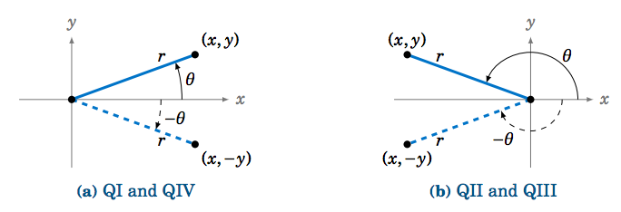
So we see that reflecting a point \((x,y) \) around the \(x\)-axis just replaces \(y \) by \(-y \). Hence:
\[\label{1.13}\sin\;(-\theta) ~ = ~ -\sin\;\theta \]
\[\label{1.14} \cos\;(-\theta) ~ = ~ \cos\;\theta \]
\[\label{1.15} \tan\;(-\theta) ~ = ~ -\tan\;\theta \]
Notice that the cosine function does not change in Equation \ref{1.14} because it depends on \(x \), and not on \(y \), for a point \((x,y) \) on the terminal side of \(\theta \).
In general, a function \(f(x) \) is an even function if \(f(-x) = f(x)\) for all \(x \), and it is called an odd function if \(f(-x) = -f(x) \) for all \(x \). Thus, the cosine function is even, while the sine and tangent functions are odd.
Replacing \(\theta \) by \(-\theta \) in Equations \ref{1.4}-\ref{1.6}, then using Equations \ref{1.13}-\ref{1.15}, gives:
\[\label{1.16}\sin\;(90^\circ - \theta) ~ = ~ \cos\;\theta \]
\[\label{1.17}\cos\;(90^\circ - \theta) ~ = ~ \sin\;\theta \]
\[\label{1.18}\tan\;(90^\circ - \theta) ~ = ~ \cot\;\theta \]
Note that Equations \ref{1.16}-\ref{1.18} extend the Cofunction Theorem from Section 1.2 to all \(\theta \), not just acute angles. Similarly, Equations \ref{1.10}-\ref{1.12} and \ref{1.13}-\ref{1.15} give:
\[\label{1.19} \sin\;(180^\circ - \theta) ~ = ~ \sin\;\theta \]
\[\label{1.20}\cos\;(180^\circ - \theta) ~ = ~ -\cos\;\theta \]
\[\label{1.21}\tan\;(180^\circ - \theta) ~ = ~ -\tan\;\theta \]
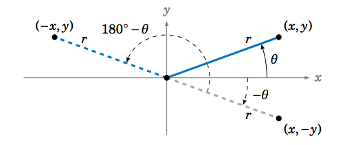
Notice that reflection around the \(y\)-axis is equivalent to reflection around the \(x\)-axis (\(\theta \mapsto -\theta\)) followed by a rotation of \(180^\circ \) (\(-\theta \mapsto -\theta + 180^\circ = 180^\circ - \theta\)), as in Figure 1.5.7.
It may seem that these geometrical operations and formulas are not necessary for evaluating the trigonometric functions, since we could just use a calculator. However, there are two reasons for why they are useful. First, the formulas work for any angles, so they are often used to prove general formulas in mathematics and other fields, as we will see later in the text. Second, they can help in determining which angles have a given trigonometric function value.
Find all angles \(0^\circ \le \theta < 360^\circ \) such that \(\sin\;\theta = -0.682 \).
Solution
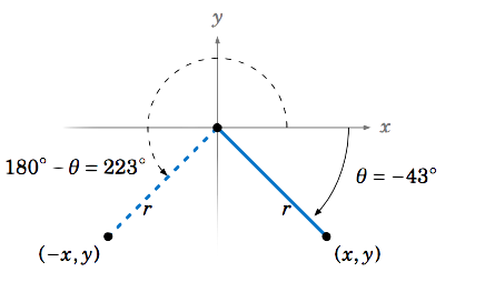
Using the \(\fbox{\(\sin^{-1}\)}\) button on a calculator with \(-0.682 \) as the input, we get \(\theta = -43^\circ \), which is not between \(0^\circ \) and \(360^\circ \). Since \(\theta = -43^\circ \) is in QIV, its reflection \(180^\circ - \theta \) around the \(y\)-axis will be in QIII and have the same sine value. But \(180^\circ - \theta = 180^\circ - (-43^\circ) = 223^\circ \) (see Figure 1.5.8). Also, we know that \(-43^\circ \) and \(-43^\circ + 360^\circ = 317^\circ \) have the same trigonometric function values. So since angles in QI and QII have positive sine values, we see that the only angles between \(0^\circ \) and \(360^\circ \) with a sine of \(-0.682 \) are \(\boxed{\theta = 223^\circ ~\text{and}~ 317^\circ}~ \).
