5.1: Graphing the Trigonometric Functions

The first function we will graph is the sine function. We will describe a geometrical way to create the graph, using the unit circle. This is the circle of radius $1$ in the $xy$-plane consisting of all points $(x,y)$ which satisfy the equation $x^2 + y^2 = 1$.

Figure $\PageIndex{1}$

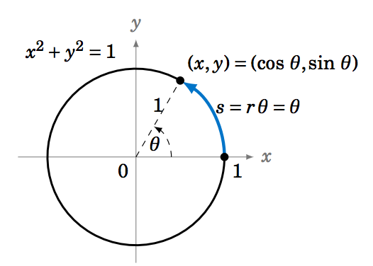
We see in Figure $\PageIndex{1}$ that any point on the unit circle has coordinates $(x,y)=(\cos\;\theta,\sin\;\theta)$, where $\theta$ is the angle that the line segment from the origin to $(x,y)$ makes with the positive $x$-axis (by definition of sine and cosine). So as the point $(x,y)$ goes around the circle, its $y$-coordinate is $\sin\;\theta$.

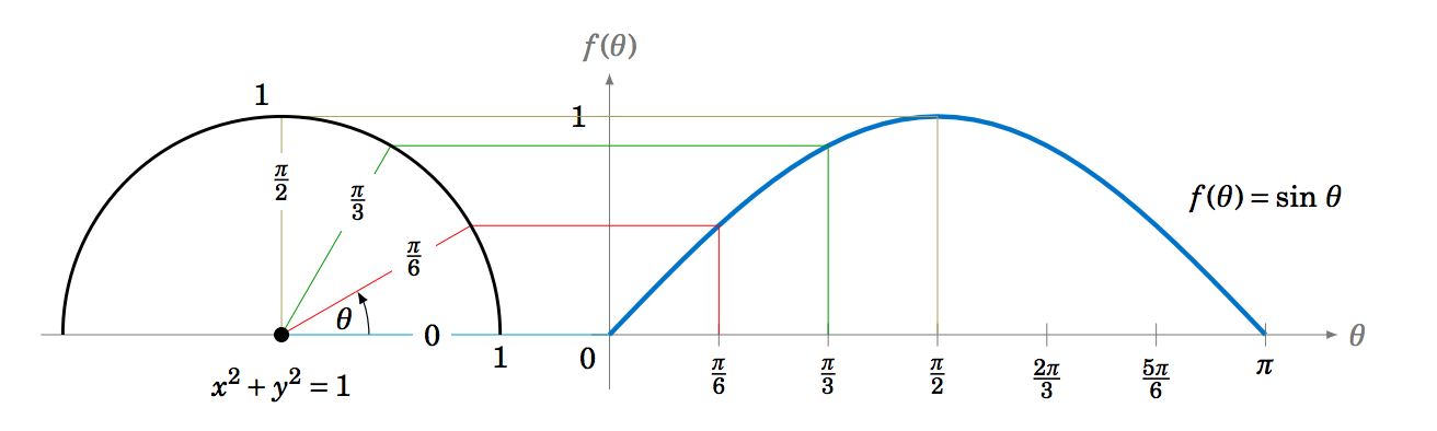
We thus get a correspondence between the $y$-coordinates of points on the unit circle and the values $f(\theta)=\sin\;\theta$, as shown by the horizontal lines from the unit circle to the graph of $f(\theta)=\sin\;\theta$ in Figure $\PageIndex{2}$ for the angles $\theta = 0$, $\tfrac{\pi}{6}$, $\tfrac{\pi}{3}$, $\tfrac{\pi}{2}$.

Figure $\PageIndex{2}$ Graph of sine function based on $y$-coordinate of points on unit circle

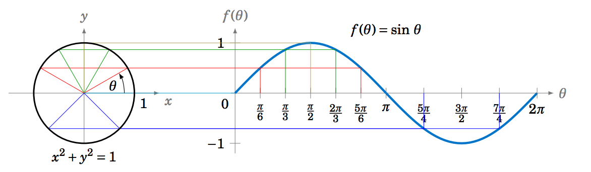
We can extend the above picture to include angles from $0$ to $2\pi$ radians, as in Figure $\PageIndex{3}$. This illustrates what is sometimes called the unit circle definition of the sine function.

Figure $\PageIndex{3}$ Unit circle definition of the sine function

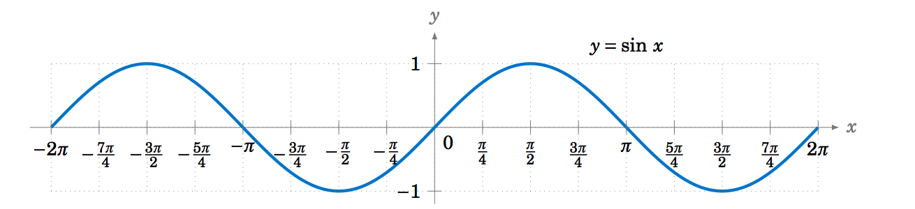
Since the trigonometric functions repeat every $2\pi$ radians ($360^\circ$), we get, for example, the following graph of the function $y=\sin\;x$ for $x$ in the interval $[-2\pi , 2\pi]$:

Figure $\PageIndex{4}$ Graph of $y = \sin x$

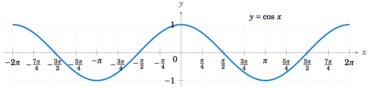
To graph the cosine function, we could again use the unit circle idea (using the $x$-coordinate of a point that moves around the circle), but there is an easier way. Recall from Section 1.5 that $\cos\;x = \sin\;(x+90^\circ)$ for all $x$. So $\cos\;0^\circ$ has the same value as $\sin\;90^\circ$, $\cos\;90^\circ$ has the same value as $\sin\;180^\circ$, $\cos\;180^\circ$ has the same value as $\sin\;270^\circ$, and so on. In other words, the graph of the cosine function is just the graph of the sine function shifted to the left by $90^\circ = \pi/2$ radians, as in Figure $\PageIndex{5}$:

Figure $\PageIndex{5}$ Graph of $y = \cos x$

To graph the tangent function, use $\tan\;x = \frac{\sin\;x}{\cos\;x}$ to get the following graph:

Figure $\PageIndex{6}$ Graph of $y = \tan x$

Recall that the tangent is positive for angles in QI and QIII, and is negative in QII and QIV, and that is indeed what the graph in Figure 5.1.6 shows. We know that $\tan\;x$ is not defined when $\cos\;x = 0$, i.e. at odd multiples of $\frac{\pi}{2}$: $x=\pm\,\frac{\pi}{2}$, $\pm\,\frac{3\pi}{2}$, $\pm\,\frac{5\pi}{2}$, etc. We can figure out what happens near those angles by looking at the sine and cosine functions. For example, for $x$ in QI near $\frac{\pi}{2}$, $\sin\;x$ and $\cos\;x$ are both positive, with $\sin\;x$ very close to $1$ and $\cos\;x$ very close to $0$, so the quotient $\tan\;x = \frac{\sin\;x}{\cos\;x}$ is a positive number that is very large. And the closer $x$ gets to $\frac{\pi}{2}$, the larger $\tan\;x$ gets. Thus, $x=\frac{\pi}{2}$ is a vertical asymptote of the graph of $y=\tan\;x$.

Likewise, for $x$ in QII very close to $\frac{\pi}{2}$, $\sin\;x$ is very close to $1$ and $\cos\;x$ is negative and very close to $0$, so the quotient $\tan\;x = \frac{\sin\;x}{\cos\;x}$ is a negative number that is very large, and it gets larger in the negative direction the closer $x$ gets to $\frac{\pi}{2}$. The graph shows this. Similarly, we get vertical asymptotes at $x=-\frac{\pi}{2}$, $x=\frac{3\pi}{2}$, and $x=-\frac{3\pi}{2}$, as in Figure $\PageIndex{6}$. Notice that the graph of the tangent function repeats every $\pi$ radians, i.e. two times faster than the graphs of sine and cosine repeat.

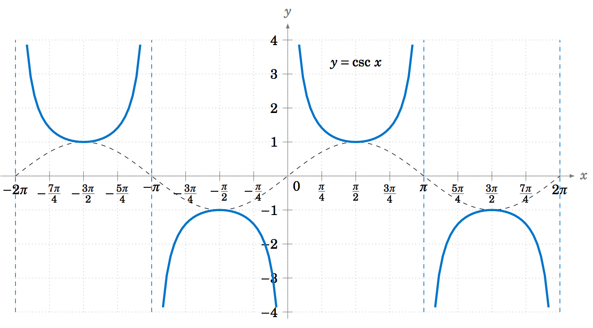
The graphs of the remaining trigonometric functions can be determined by looking at the graphs of their reciprocal functions. For example, using $\csc\;x = \frac{1}{\sin\;x}$ we can just look at the graph of $y=\sin\;x$ and invert the values. We will get vertical asymptotes when $\sin\;x=0$, namely at multiples of $\pi$: $x=0$, $\pm\,\pi$, $\pm\,2\pi$, etc. Figure $\PageIndex{7}$ shows the graph of $y=\csc\;x$, with the graph of $y=\sin\;x$ (the dashed curve) for reference.

Figure $\PageIndex{7}$ Graph of $y = \csc x$

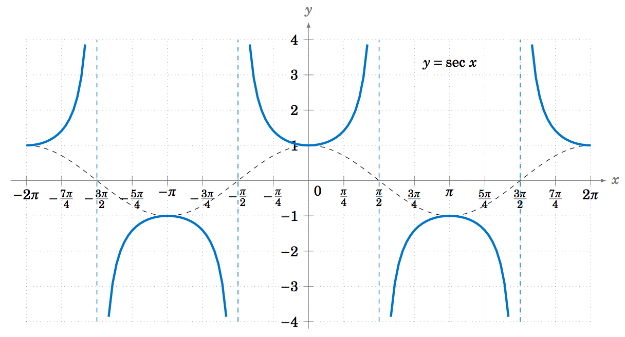
Likewise, Figure $\PageIndex{8}$ shows the graph of $y=\sec\;x$, with the graph of $y=\cos\;x$ (the dashed curve) for reference. Note the vertical asymptotes at $x=\pm\,\frac{\pi}{2}$, $\pm\,\frac{3\pi}{2}$. Notice also that the graph is just the graph of the cosecant function shifted to the left by $\frac{\pi}{2}$ radians.

Figure $\PageIndex{8}$ Graph of $y = \sec x$

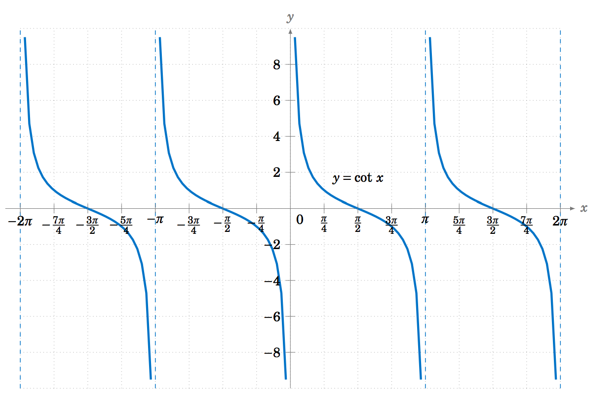
The graph of $y=\cot\;x$ can also be determined by using $\cot\;x = \frac{1}{\tan\;x}$. Alternatively, we can use the relation $\cot\;x = -\tan\;(x+90^\circ)$ from Section 1.5, so that the graph of the cotangent function is just the graph of the tangent function shifted to the left by $\frac{\pi}{2}$ radians and then reflected about the $x$-axis, as in Figure $\PageIndex{9}$:

Figure $\PageIndex{9}$ Graph of $y = \cot x$

Example $\PageIndex{1}$

Draw the graph of $y=-\sin\;x$ for $0 \le x \le 2\pi$.

Solution:

Multiplying a function by $-1$ just reflects its graph around the $x$-axis. So reflecting the graph of $y=\sin\;x$ around the $x$-axis gives us the graph of $y=-\sin\;x$:

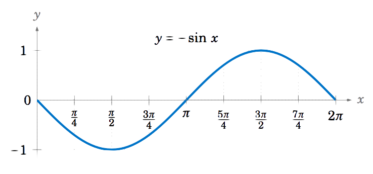
\noindent Note that this graph is the same as the graphs of $y=\sin\;(x \pm \pi)$ and $y=\cos\;(x+\frac{\pi}{2})$.

It is worthwhile to remember the general shapes of the graphs of the six trigonometric functions, especially for sine, cosine, and tangent. In particular, the graphs of the sine and cosine functions are called sinusoidal curves. Many phenomena in nature exhibit sinusoidal behavior, so recognizing the general shape is important.

Example $\PageIndex{2}$

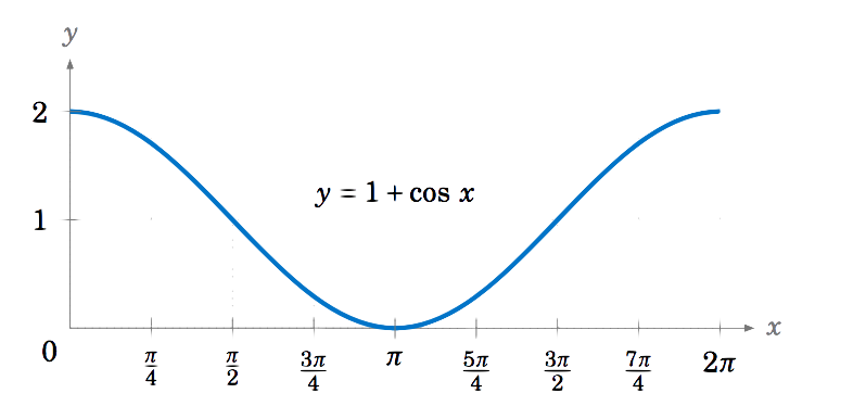
Draw the graph of $y=1+\cos\;x$ for $0 \le x \le 2\pi$.

Solution

Adding a constant to a function just moves its graph up or down by that amount, depending on whether the constant is positive or negative, respectively. So adding $1$ to $\cos\;x$ moves the graph of $y=\cos\;x$ upward by $1$, giving us the graph of $y=1+\cos\;x$: