6.6: Making New Kinds of Graphs from Existing Graphs

Turning Attributes into Relations

At the beginning of this chapter we looked at the "data structures" most commonly used in network analysis. One was the node-by-node square matrix, to record the relations between pairs of actors; and its more general "multiplex" form to record multiple relations among the same set of actors. The other was the rectangular matrix. This "actor by attribute" matrix is most commonly used to record information about the variable properties of each node.

Network analysis often finds it useful to see actor attributes as actually indicating the presence, absence, or strength of "relations" among actors. Suppose two persons have the same gender. To the non-network analyst, this may represent a statistical regularity that describes the frequencies of scores on a variable. A network analyst, though, might interpret the same data a bit differently. A network analyst might, instead, say "these two persons share the relation of having the same gender".

Both interpretations are, of course, entirely reasonable. One emphasizes the attributes of individuals (here are two persons, each is a woman); one emphasizes the relation between them (here are two persons who are related by sharing the same social role).

It's often the case that network researchers, whoa re pre-disposed to see the world in "relational" terms, want to turn "attribute" data in "relational" data for their analyses.

Data>Attribute is a tool that creates an actor-by-actor relational matrix from the scores on a single attribute vector. Suppose that we had an attribute vector stored in a UCINET file (other vectors could also be in the file, but this algorithm operates on a single vector), that measured whether each of 100 large donors had given funds in support of (+1) or in opposition to (-1) a given ballot proposition. Those who made no contribution are coded zero.

We might like to create a new matrix that identifies pairs of actors who shared support or shared opposition to the ballot initiative, or who took opposite positions. That is, for each pair of actors, the matrix element is "1" if the actors jointly supported or jointly opposed the proposition, "-1" if one supported and the other opposed, and zero otherwise (if either or both made no contribution).

Using the Data>Attribute tool, we can form a new square (actor-by-actor) matrix from the scores of actors on one attribute in a number of ways. The Exact Matches choice will produce a "1" when two actors have exactly the same score on the attribute, and zero otherwise. The Difference choice will create a new matrix where the elements are the differences between the attribute scores of each pair of actors (alternatively, the Absolute Difference, or Squared Difference choices will yield positively valued measures of the distance between the attribute scores of each pair of actors). The Sum choice yields a score for each pair that is equal to the sum of their attribute scores. In our current example, the Product choice (that is, multiply the score of actor i times the score of actor j, and enter the result) would yield a score of "1" if two actors shared either support or opposition, "-1" if they took opposed stands on the issue, or "0" if either did not take a position.

The Data>Attribute tool can be very useful for conceptually turning attributes into relations, so that their association with other relations can be studied.

Data>Affiliations extends the idea of turning attributes into relations to the case where we want to consider to multiple attributes. Probably the most common situations of this type are where the multiple "attributes" we have measured are "repeated measures" of some sort. Davis, for example, measured the presence of a number of persons (rows) at a number of parties (attributes or columns). From these data, we might be interested in the similarity of all pairs of actors (how many times where they co-present at the same event?), or how similar were the parties (how much of the attendance of each pair of parties were the same people?).

The example of donors to political campaigns can be seen in the same way. We might collect information on whether political donors (rows) had given funds against or for a number of different ballot propositions (columns). From this rectangular matrix, we might be interested in forming a square actor-by-actor matrix (how often to each pair of actors donate to the same campaigns?); we might be interested in forming a square campaign-by-campaign matrix (how similar are the campaigns in terms of their constituencies?).

The Data>Affiliations algorithm begins with a rectangular (actor-by-affiliate) matrix, and asks you to select whether the new matrix is to be formed by rows (i.e. actor-by-actor) or columns (i.e. attribute-by-attribute).

There are different ways in which we could form the entries of the new matrix. UCINET provides two methods: Cross-Products or Minimums. These approaches produce the same result for binary data, but different results for valued data.

Let's look at the binary case first. Consider two actors "A" and "B" who have made contributions (or not) to each of 5 political campaigns, as in Figure 6.7.

	Campaign 1	Campaign 2	Campaign 3	Campaign 4	Campaign 5
A	0	0	1	1	1
B	0	1	1	0	1

Figure 6.7: Donations of two donors to five political campaigns (binary data)

The Cross-Products method multiplies each of A's scores by the corresponding score for B, and then sums across the columns (if we were creating a campaign-by-campaign matrix, the logic is exactly the same, but would operate by multiplying columns, and summing across rows). Here, this results in: \(\left( 0 * 0 \right) + \left( 0 * 1 \right) + \left( 1 * 1 \right) + \left( 1 * 0 \right) + \left( 1 * 1 \right) = 2\). That is, actors A and B have two instances where they both supported a campaign.

The Minimums method examines the entries of A and B for Campaign 1, and selects the lowest score (zero). It then does this for the other campaigns (resulting in 0, 1, 0, 1) and sums. With binary data, the results will be the same by either method.

With valued data, the methods do not produce the same results; they get at rather different ideas.

Suppose that we had measured whether A and B supported (+1) , took no position on (0), or opposed (-1) each of the five campaigns. This is the simplest possible "valued" data, but the ideas hold for valued scales with wider ranges, and with all positive values, as well. Now, our data might look like those in Figure 6.8.

	Campaign 1	Campaign 2	Campaign 3	Campaign 4	Campaign 5
A	-1	0	1	-1	1
B	-1	1	1	0	-1

Figure 6.8: Donations of two donors for or against five political campaigns (valued data)

Both A and B took the same position on two issues (both opposed on one, both supporting another). On two campaigns (2, 4), one took no stand. On issue number 5, the two actors took opposite positions.

The Cross-Products method yields: \(\left( -1 * -1 \right) + \left( 0 * 1 \right) + \left( 1 * 1 \right) + \left( -1 * 0 \right) + \left( 1 * -1 \right)\). That is: 1 + 0 + 1 + 0 + -1, or 1. The two actors have a "net" agreement of 1 (they took the same position on two issues, but opposed positions on one issue).

The Minimums method yields: -1 + 0 + 1 - 1 - 1 or -2. In this example, this is difficult to interpret, but can be seen as the net number of times either member of the pair opposed an issue. The minimums method produces results that are easier to interpret when all values are positive. Suppose we re-coded the data to be: 0 = opposed, 1 = neutral, and 2 = favor. The minimums method would then produce 0 + 1 + 2 + 0 + 0 = 3. This might bee seen as the extent to which the pair of actors jointly supported the five campaigns.

Turning Relations into Attributes

Suppose that we had a simple directed relation, represented as a matrix as in Figure 6.9.

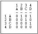
Figure 6.9: Linegraph example matrix

This is easier to see as a graph, as in Figure 6.10.

Figure 6.10: Linegraph example graph

Now suppose that we are really interested in describing and thinking about the relations, and the relations among the relations - rather than the actors, and the relations among them. That sounds odd, I realize. Let me put it a different way. We can think about the graph in Figure 6.5 as composed of four relations (A to B, B to C, C to D, and A to C). These relations are connected by having actors in common (e.g. the A to B and the B to C relations have the actor B in common). That is, we can think about relations as being "adjacent" when they share actors, just as we can think about actors being adjacent when they share relations.

Transform>Incidence is an algorithm that changes the way we look at a directed graph from "actors connected by relations" to "relations connected by actors". This is sometimes just a semantic trick. But, sometimes it's more than that - our theory of the social structure may actually be one about which relations are connected, not which actors are connected. If we apply the Transform>Incidence algorithm to the data in Figures 6.4 and 6.5, we get the result in Figure 6.11.

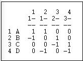
Figure 6.11: Incidence matrix of Figure 6.10

Each row is an actor. Each column is now a relation (the relations are numbered 1 through 4). A positive entry indicates that an actor is the source of a directed relation. For example, actor A is the origin of the relation "1" that connects A to B, and is a source of the relation "2" that connects actor A to actor D. A negative entry indicates that an actor is the "sink" or recipient of a directed relation. For example, actor C is the recipient in relation "3" (which connects actor B to actor C), and the source of relation "4" (which connects actor C to actor D).

The "incidence" matrix here then shows how actors are connected to relationships. By examining the rows, we can characterize how much, and in what ways actors are embedded in relations. One actor may have few entries - a near isolate; another may have many negative and few positive entries - a "taker" rather than a "giver". By examining the columns, we get a description of which actors are connected, in which way, by each of the relations in the graph.

Focusing on the Relations, Instead of the Actors

Turning an actor-by-actor adjacency matrix into an actor-by-relation incidence graph takes us part of the way toward focusing on relations rather than actors. We can go further.

Transform>Linegraph converts an actor-by-actor matrix (like Figure 6.4) into a full relation-by-relation matrix. Figure 6.12 shows the results of applying it to the example data.

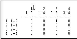
Figure 6.12: Linegraph matrix

We again have a square matrix. This time, though, it describes which relations in the graph are "adjacent to" which other relations. Two relations are adjacent if they share an actor. For example, relation "1" (the tie between actors 1 and 2, or A and B) is adjacent to the relation "3" (the tie between actors 2 and 3, or B and C). Note that the "adjacency" here is directional - relation 1 is a source of relation 3. We could also apply this approach to symmetric or simple graphs to describe which relations are simply adjacent in an un-directed way.

A quick glance at the linegraph matrix is suggestive. It is very sparse in this example - most of the relations are not sources of other relations. The maximum degree of each entry is 1 - no relation is the source of multiple relations. While there may be a key or central actor (A), it's not so clear that there is a single central relation.

To be entirely honest, most social network analysts do (much of the time) think about actors connected to actors by relations, rather than relations connecting actors, or relations connecting relations. But changing our point of view to put the relations first, and the actors second is, in many ways, a more distinctively "sociological" way of looking at networks. Transforming actor-by-actor data into relation-by-relation data can yield some interesting insights about social structures.