
7.2: Connection

( \newcommand{\kernel}{\mathrm{null}\,}\)
Since networks are defined by their actors and the connections among them, it is useful to begin our description of networks by examining these very simple properties. Focusing first on the network as a whole, one might be interested in the number of actors, the number of connections that are possible, and the number of connections that are actually present. Differences in the size of networks, and how connected the actors are tell us two things about human populations that are critical. Small groups differ from large groups in many important ways - indeed, population size is one of the most critical variables in all sociological analyses. Differences in how connected the actors in a population are may be a key indicator of the "cohesion", "solidarity", "moral density", and "complexity" of the social organization of a population.
Individuals, as well as whole networks, differ in these basic demographic features. Individual actors may have many or few ties. Individuals may be "sources" of ties, "sinks" (actors that receive ties, but don't send them), or both. These kinds of very basic differences among actors' immediate connections may be critical in explaining how they view the world, and how the world views them. The number and kinds of ties that actors have are a basis for similarity or dissimilarity to other actors - and hence to possible differentiation and stratification. The number and kinds of ties that actors have are keys to determining how much their embeddedness in the network constrains their behavior, and the range of opportunities, influence, and power that they have.
Basic Demographics
Network size. The size of a network is often very important. Imagine a group of 12 students in a seminar. It would not be difficult for each of the students to know each of the others fairly well, and build up exchange relationships (e.g. sharing reading notes). Now imagine a large lecture class of 300 students. It would be extremely difficult for any student to know all of the others, and it would be virtually impossible for there to be a single network for exchanging reading notes. Size is critical for the structure of social relations because of the limited resources and capacities that each actor has for building and maintaining ties. Our example network has ten actors. Usually the size of a network is indexed simply by counting the number of nodes.
In any network there are (k∗k−1) unique ordered pairs of actors (that is AB is different from BA, and leaving aside self-ties), where k is the number of actors. You may wish to verify this for yourself with some small networks. So, in our network of 10 actors, with directed data, there are 90 logically possible relationships. If we had undirected, or symmetric, ties, the number would be 45, since the relationship AB would be the same as BA. The number of logically possible relationships then grows exponentially as the number of actors increases linearly. It follows from this that the range of logically possible social structures increases (or, by one definition, "complexity" increases) exponentially with size.
Actor degree. The number of actors places an upper limit on the number of connections that each individual can have (k−1). For networks of any size, though, few - if any - actors approach this limit. It can be quite useful to examine the distribution of actor degree. The distribution of how connected individual actors are can tell use a good bit about the social structure.
Since the data in our example are asymmetric (that is, directed ties), we can distinguish between ties being sent and ties being received. Looking at the density for each row and for each column can tell us a good bit about the way in which actors are embedded in the overall density.
Tools>Univariate Stats provides quick summaries of the distribution of actor's ties.
Let's first examine these statistics for the rows, or out-degree of actors.
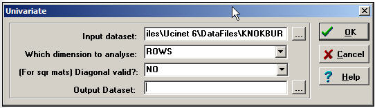
Figure 7.3: Dialog for Tools>Univariate Stats
Produces this result:
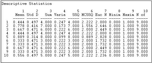
Figure 7.4: Out-degree statistics for Knoke information exchange
Statistics on the rows tell us about the role that each actor plays as a "source" of ties (in a directed graph). The sum of the connections from the actor to others (e.g. actor #1 sends information to four others) is called the out-degree of the point (for symmetric data, of course, each node simply has degree, as we cannot distinguish in-degree from out-degree). The degree of points is important because it tells us how many connections an actor has. With out-degree, it is usually a measure of how influential the actor may be.
We can see that actor #5 sends ties to all but one of the remaining actors; actors #6, #7, and #9 send information to only three other actors. Actors #2, #3, #5, and #8 are similar in being sources of information for large portions of the network; actors #1, #6, #7 and #9 are similar in not being sources of information. We might predict that the first set of organizations will have specialized divisions for public relations, the latter set might not. Actors in the first set have a higher potential to be influential; actors in the latter set have lower potential to be influential; actors in "the middle" will be influential if they are connected to the "right" other actors, otherwise, they might have very little influence. So, there is variation in the roles that these organizations play as sources of information. We can norm this information (so we can compare it to other networks of different sizes, by expressing the out-degree of each point as a proportion of the number of elements in the row; that is, calculating the mean). Actor #10, for example, sends ties to 56% of the remaining actors. This is a figure we can compare across networks of different sizes.
Another way of thinking about each actor as a source of information is to look at the row-wise variance or standard deviation. We note that actors with very few out-ties, or very many out-ties, have less variability than those with medium levels of ties. This tells us something: those actors with ties to almost everyone else, or with ties to almost no-one else are more "predictable" in their behavior toward any given other actor than those with intermediate numbers of ties. In a sense, actors with many ties (at the center of a network) and actors at the periphery of a network (few ties) have patterns of behavior that are more constrained and predictable. Actors with only some ties can vary more in their behavior, depending on to whom they are connected.
If we were examining a valued relation instead of a binary one, the meaning of the "sum", "mean", and "standard deviation" of actors' out-degree would differ. If the values of the relations are all positive and reflect the strength or probability of a tie between nodes, these statistics would have the easy interpretations as the sum of the strengths, the average strength, and variation in strength.
It's useful to examine the statistics for in-degree, as well (look at the data column-wise). Now, we are looking at the actors as "sinks" or receivers of information. The sum of each column in the adjacency matrix is the in-degree of the point. That is, how many other actors send information or ties to the one we are focusing on. Actors that receive information from many sources may be prestigious (other actors want to be known by the actor, so they send information). Actors that receive information from many sources may also be more powerful - to the extent that "knowledge is power". But, actors that receive a lot of information could also suffer from "information overload" or "noise and interference" due to contradictory messages from different sources.
Here are the results of Tools>Univariate Stats when we select "column" instead of "row".
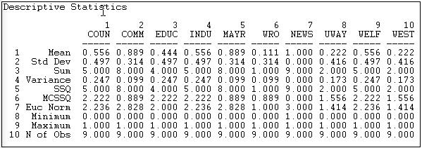
Figure 7.5: In-degree statistics for Knoke information exchange
Looking at the means, we see that there is a lot of variation in information receiving - more than for information sending. We see that actors #2, #5, and #7 are very high. #2 and #5 are also high in sending information - so perhaps they act as "communicators" and "facilitators" in the system. Actor #7 receives a lot of information, but does not send a lot. Actor #7, as it turns out, is an "information sink" - it collects facts, but it does not create them (at least we hope so, since actor #7 is a newspaper). Actors #6, #8, and #10 appear to be "out of the loop" - that is, they do not receive information from many sources directly. Actor #6 also does not send much information - so #6 appears to be something of an "isolate". Actors #8 and #10 send relatively more information than they receive. One might suggest that they are "outsiders" who are attempting to be influential, but may be "clueless".
We can learn a great deal about a network overall, and about the structural constraints on individual actors, and even start forming some hypotheses about social roles and behavioral tendencies, just by looking at the simple adjacencies and calculating a few very basic statistics. Before discussing the slightly more complex idea of distance, there are a couple other aspects of "connectedness" that are sometimes of interest.
Density
The density of a binary network is simply the proportion of all possible ties that are actually present. For a valued network, density is defined as the sum of the ties divided by the number of possible ties (i.e. the ratio of all tie strength that is actually present to the number of possible ties). The density of a network may give us insights into such phenomena as the speed at which information diffuses among the nodes, and the extent to which actors have high levels of social capital and/or social constraint.
Network>Cohesion>Density is a quite powerful tool for calculating densities. Its dialog is shown in Figure 7.6.
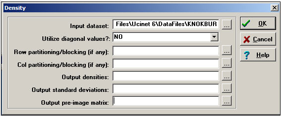
Figure 7.6: Dialog for Network>Cohesion>Density
To obtain densities for a matrix (as we are doing in this example), we simply need a dataset. Usually self-ties are ignored in computing density (but there are circumstances where you might want to include them). The Network>Cohesion>Density algorithm also can be used to calculate the densities within partitions or blocks by specifying the file name of an attribute data set that contains the node name and partition number. That is, the density tool can be used to calculate within and between block densities for data that are grouped. One might, for example, partition the Knoke data into "public" and "private" organizations, and examine the density of information exchange within and between types.
For our current purposes, we won't block or partition the data. Here's the result of the dialog above.
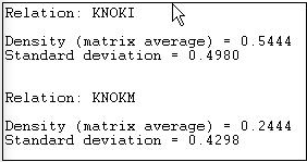
Figure 7.7: Density of Knoke information network
Since the Knoke data set contains two matrices, separate reports for each relation (KNOKI and KNOKM) are produced.
The density of the information exchange matrix is 0.5444. That is, 54% of all the possible ties are present. The standard deviation of the entries in the matrix is also given. For binary data, the standard deviation is largely irrelevant - as the standard deviation of a binary variable is a function of its mean.
Reachability
An actor is "reachable" by another if there exists any set of connections by which we can trace from the source to the target actor, regardless of how many others fall between them. If the data are asymmetric or directed, it is possible that actor A can reach actor B, but that actor B cannot reach actor A. With symmetric or undirected data, of course, each pair of actors either are or are not reachable to one another. If some actors in a network cannot reach others, there is the potential of a division of the network. Or, it may indicate that the population we are studying is really composed of more than one sub-populations.
In the Knoke information exchange dataset, it turns out that all actors are reachable by all others. This is something that you can verify by eye. See if you can find any pair of actors in the diagram such that you cannot trace from the first to the second along arrows all headed in the same direction (don't waste a lot of time on this, there is no such pair!). For the Knoke "M" relation, it turns out that not all actors can "reach" all other actors. Here's the output of Network>Cohesion>Reachability from UCINET.

Figure 7.8: Reachability of Knoke "I" and "M" relations
So, there exists a directed "path" from each organization to each other actor for the flow of information, but not for the flow of money. Sometimes "what goes around comes around", and sometimes it doesn't!
Connectivity
Adjacency tells us whether there is a direct connection from one actor to another (or between two actors for undirected data). Reachability tells us whether two actors are connected or not by way of either a direct or an indirect pathway of any length.
Network>Cohesion>Point Connectivity calculates the number of nodes that would have to be removed in order for one actor to no longer be able to reach another. If there are many different pathways that connect two actors, they have high "connectivity" in the sense that there are multiple ways for a signal to reach from one to the other. Figure 7.9 shows the point connectivity for the flow of information among the 10 Knoke organizations.

Figure 7.9: Point connectivity of Knoke information exchange
The result again demonstrates the tenuousness of organization 6's connection as both a source (row) or receiver (column) of information. To get its message to most other actors, organization 6 has alternative; should a single organization refuse to pass along information, organization 6 would receive none at all! Point connectivity can be a useful measure to get at notions of dependency and vulnerability.