14.3: Finding Equivalence Sets
- Page ID
- 7737
\( \newcommand{\vecs}[1]{\overset { \scriptstyle \rightharpoonup} {\mathbf{#1}} } \)
\( \newcommand{\vecd}[1]{\overset{-\!-\!\rightharpoonup}{\vphantom{a}\smash {#1}}} \)
\( \newcommand{\id}{\mathrm{id}}\) \( \newcommand{\Span}{\mathrm{span}}\)
( \newcommand{\kernel}{\mathrm{null}\,}\) \( \newcommand{\range}{\mathrm{range}\,}\)
\( \newcommand{\RealPart}{\mathrm{Re}}\) \( \newcommand{\ImaginaryPart}{\mathrm{Im}}\)
\( \newcommand{\Argument}{\mathrm{Arg}}\) \( \newcommand{\norm}[1]{\| #1 \|}\)
\( \newcommand{\inner}[2]{\langle #1, #2 \rangle}\)
\( \newcommand{\Span}{\mathrm{span}}\)
\( \newcommand{\id}{\mathrm{id}}\)
\( \newcommand{\Span}{\mathrm{span}}\)
\( \newcommand{\kernel}{\mathrm{null}\,}\)
\( \newcommand{\range}{\mathrm{range}\,}\)
\( \newcommand{\RealPart}{\mathrm{Re}}\)
\( \newcommand{\ImaginaryPart}{\mathrm{Im}}\)
\( \newcommand{\Argument}{\mathrm{Arg}}\)
\( \newcommand{\norm}[1]{\| #1 \|}\)
\( \newcommand{\inner}[2]{\langle #1, #2 \rangle}\)
\( \newcommand{\Span}{\mathrm{span}}\) \( \newcommand{\AA}{\unicode[.8,0]{x212B}}\)
\( \newcommand{\vectorA}[1]{\vec{#1}} % arrow\)
\( \newcommand{\vectorAt}[1]{\vec{\text{#1}}} % arrow\)
\( \newcommand{\vectorB}[1]{\overset { \scriptstyle \rightharpoonup} {\mathbf{#1}} } \)
\( \newcommand{\vectorC}[1]{\textbf{#1}} \)
\( \newcommand{\vectorD}[1]{\overrightarrow{#1}} \)
\( \newcommand{\vectorDt}[1]{\overrightarrow{\text{#1}}} \)
\( \newcommand{\vectE}[1]{\overset{-\!-\!\rightharpoonup}{\vphantom{a}\smash{\mathbf {#1}}}} \)
\( \newcommand{\vecs}[1]{\overset { \scriptstyle \rightharpoonup} {\mathbf{#1}} } \)
\( \newcommand{\vecd}[1]{\overset{-\!-\!\rightharpoonup}{\vphantom{a}\smash {#1}}} \)
\(\newcommand{\avec}{\mathbf a}\) \(\newcommand{\bvec}{\mathbf b}\) \(\newcommand{\cvec}{\mathbf c}\) \(\newcommand{\dvec}{\mathbf d}\) \(\newcommand{\dtil}{\widetilde{\mathbf d}}\) \(\newcommand{\evec}{\mathbf e}\) \(\newcommand{\fvec}{\mathbf f}\) \(\newcommand{\nvec}{\mathbf n}\) \(\newcommand{\pvec}{\mathbf p}\) \(\newcommand{\qvec}{\mathbf q}\) \(\newcommand{\svec}{\mathbf s}\) \(\newcommand{\tvec}{\mathbf t}\) \(\newcommand{\uvec}{\mathbf u}\) \(\newcommand{\vvec}{\mathbf v}\) \(\newcommand{\wvec}{\mathbf w}\) \(\newcommand{\xvec}{\mathbf x}\) \(\newcommand{\yvec}{\mathbf y}\) \(\newcommand{\zvec}{\mathbf z}\) \(\newcommand{\rvec}{\mathbf r}\) \(\newcommand{\mvec}{\mathbf m}\) \(\newcommand{\zerovec}{\mathbf 0}\) \(\newcommand{\onevec}{\mathbf 1}\) \(\newcommand{\real}{\mathbb R}\) \(\newcommand{\twovec}[2]{\left[\begin{array}{r}#1 \\ #2 \end{array}\right]}\) \(\newcommand{\ctwovec}[2]{\left[\begin{array}{c}#1 \\ #2 \end{array}\right]}\) \(\newcommand{\threevec}[3]{\left[\begin{array}{r}#1 \\ #2 \\ #3 \end{array}\right]}\) \(\newcommand{\cthreevec}[3]{\left[\begin{array}{c}#1 \\ #2 \\ #3 \end{array}\right]}\) \(\newcommand{\fourvec}[4]{\left[\begin{array}{r}#1 \\ #2 \\ #3 \\ #4 \end{array}\right]}\) \(\newcommand{\cfourvec}[4]{\left[\begin{array}{c}#1 \\ #2 \\ #3 \\ #4 \end{array}\right]}\) \(\newcommand{\fivevec}[5]{\left[\begin{array}{r}#1 \\ #2 \\ #3 \\ #4 \\ #5 \\ \end{array}\right]}\) \(\newcommand{\cfivevec}[5]{\left[\begin{array}{c}#1 \\ #2 \\ #3 \\ #4 \\ #5 \\ \end{array}\right]}\) \(\newcommand{\mattwo}[4]{\left[\begin{array}{rr}#1 \amp #2 \\ #3 \amp #4 \\ \end{array}\right]}\) \(\newcommand{\laspan}[1]{\text{Span}\{#1\}}\) \(\newcommand{\bcal}{\cal B}\) \(\newcommand{\ccal}{\cal C}\) \(\newcommand{\scal}{\cal S}\) \(\newcommand{\wcal}{\cal W}\) \(\newcommand{\ecal}{\cal E}\) \(\newcommand{\coords}[2]{\left\{#1\right\}_{#2}}\) \(\newcommand{\gray}[1]{\color{gray}{#1}}\) \(\newcommand{\lgray}[1]{\color{lightgray}{#1}}\) \(\newcommand{\rank}{\operatorname{rank}}\) \(\newcommand{\row}{\text{Row}}\) \(\newcommand{\col}{\text{Col}}\) \(\renewcommand{\row}{\text{Row}}\) \(\newcommand{\nul}{\text{Nul}}\) \(\newcommand{\var}{\text{Var}}\) \(\newcommand{\corr}{\text{corr}}\) \(\newcommand{\len}[1]{\left|#1\right|}\) \(\newcommand{\bbar}{\overline{\bvec}}\) \(\newcommand{\bhat}{\widehat{\bvec}}\) \(\newcommand{\bperp}{\bvec^\perp}\) \(\newcommand{\xhat}{\widehat{\xvec}}\) \(\newcommand{\vhat}{\widehat{\vvec}}\) \(\newcommand{\uhat}{\widehat{\uvec}}\) \(\newcommand{\what}{\widehat{\wvec}}\) \(\newcommand{\Sighat}{\widehat{\Sigma}}\) \(\newcommand{\lt}{<}\) \(\newcommand{\gt}{>}\) \(\newcommand{\amp}{&}\) \(\definecolor{fillinmathshade}{gray}{0.9}\)With binary data, numerical algorithms are used to search for classes of actors that satisfy the mathematical definitions of automorphic equivalence. Basically, the nodes of a graph are exchanged, and the distances among all pairs of actors in the new graph are compared to the original graph. When the new graph and the old graph have the same distances among nodes, the graphs are isomorphic, and the "swapping" that was done identifies the isomorphic sub-graphs.
One approach to binary data, "all permutations," (Network>Roles & Positions>Automorphic>All Permutations) literally compares every possible swapping of nodes to find isomorphic graphs. With even a small graph, there are a very large number of such alternatives, and the computation is extensive. An alternative approach with the same intent ("optimization by tabu search") (Network>Roles & Positions>Exact>Optimization) can much more quickly sort nodes into a user-defined number of partitions in such a way as to maximize automorphic equivalence. There is no guarantee, however, that the number of partitions (equivalence classes) chosen is "correct," or that the automorphisms identified are "exact." For larger data sets, and where we are willing to entertain the idea that two sub-structures can be "almost" equivalent, optimization is a very useful method.
When we have measures of the strength, cost, or probability of relations among nodes (i.e. valued data), exact automorphic equivalence is far less likely. It is possible, however, to identify classes of approximately equivalent actors on the basis of their profile of distance to all other actors. The "equivalence of distances" method (Network>Roles & Positions>Automorphic>MaxSim) produces measures of the degree of automorphic equivalence for each pair of nodes, which can be examined by clustering and scaling methods to identify approximate classes. This method can also be applied to binary data by first turning binary adjacency into some measure of graph distance (usually, geodesic distance).
Let's look at these in a little more detail, with some examples.
All Permutations (i.e. Brute Force)
The automorphisms in a graph can be identified by the brute force method of examining every possible permutation of the graph. With a small graph, and a fast computer, this is a useful thing to do. Basically, every possible permutation of the graph is examined to see if it has the same tie structure as the original graph. For graphs of more than a few actors, the number of permutations that need to be compared becomes extremely large.
Let's use Networks>Roles & Positions>Automorphic>All Permutations to search the Wasserman-Faust network shown in Figure 14.1.
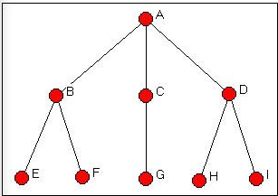
Figure 14.1: Wasserman-Faust network
The results of Networks>Roles & Positions>Automorphic>All Permutations for this graph are shown in Figure 14.2.
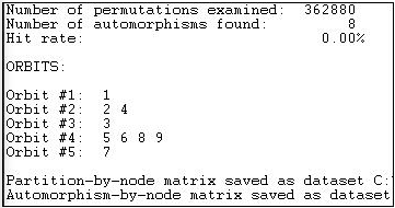
Figure 14.2: Automorphic equivalences by all permutations for the Wasserman-Faust network
The algorithm examined over three hundred sixty two thousand possible permutations of the graph. The isomorphism classes that it located are called "orbits." And, the results correspond to our logical analysis (chapter 12). There are five "types" of actors who are embedded at equal distances from other sets of actors: actor A (orbit 1), actor C (orbit 3), and actor G (orbit 7) are unique. Actors B and D form a class of actors who can be exchanged if members of other classes are also exchanged; actors E, F, H, and I (5, 6, 8, and 9) also form a class of exchangeable actors.
Note that automorphism classes identify groups of actors who have the same pattern of distance from other actors, rather than the "sub-structures" themselves (in this case, the two branches of the tree.
Optimization by Tabu Search
For larger graphs, direct search for all equivalencies is impractical both because it is computationally intensive, and because exactly equivalent actors are likely to be rare.
Network>Roles & Positions>Exact>Optimization provides a numerical tool for finding the best approximations to a user-selected number of automorphism classes. In using this method, it is important to explore a range of possible numbers of partitions (unless one has a prior theory about this), to determine how many partitions are useful. Having selected a number of partitions, it is useful to re-run the algorithm a number of times to insure that a global, rather than local minimum has been found.
The method begins by randomly allocating nodes to partitions. A measure of badness of fit is constructed by calculating the sums of squares for each row and each column within each block, and calculating the variance of these sums of squares. These variances are then summed across the blocks to construct a measure of badness of fit. Search continues to find an allocation of actors to partitions that minimizes this badness of fit statistic.
What is being minimized is a function of the dissimilarity of the variance of scores within partitions. That is, the algorithm seeks to group together actors who have similar amounts of variability in their row and column scores within blocks. Actors who have similar variability probably have similar profiles of ties sent and received within, and across blocks -- though they do not necessarily have the same ties to the same other actors, they are likely to have ties of the same distance to actors in other classes.
Let's examine the Knoke bureaucracies information exchange network again, this time looking for automorphisms. In the Knoke information data there are no exact automorphisms. This is not really surprising, given the complexity of the pattern (and particularly if we distinguish in-ties from out-ties) of connections.
We ran the routine a number of times, requesting partitions into different numbers of classes. Figure 14.3 summarizes the "badness of fit" of the models.
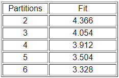
Figure 14.3: Fit of automorphic equivalence models to Knoke information network
There is no "right" answer about how many classes there are. There are two trivial answers: those that group all the cases together into one partition and those that separate each case into its own partition. In between, one might want to follow the logic of the "scree" plot from factor analysis to select a meaningful number of partitions. Look first at the results for three partitions (Figure 14.4).
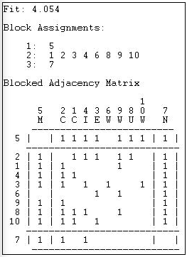
Figure 14.4: 3-class automorphic equivalence solution for the Knoke information network
At this level of approximate equivalence, there are three classes - two individuals and one large group. The newspaper (actor 7) has low rates of sending (row) and high rates of receiving (column); the mayor (actor 5) has high rates of sending and high rates of receiving. With only three classes, the remainder of the actors are grouped into an approximate class with roughly equal (and higher) variability of both sending and receiving.
Because automorphic equivalence actually operates on the profile of distances of actors, it tends to identify groupings of actors who have similar patterns of in and out degree. This goes beyond structural equivalence (which emphasizes ties to exactly the same other actors) to a more general and fuzzier idea that two actors are equivalent if they are similarly embedded. The emphasis shifts from individual position, to the role of the position in the structure of the whole graph.
Equivalence of Distances (MaxSim)
When we have information on the strength, cost, or probability of relations (i.e. valued data), exact automorphic equivalence could be expected to be extremely rare. But, since automorphic equivalence emphasizes the similarity in the profile of distances of actors from others, the idea of approximate equivalence can be applied to valued data. Network>Roles & Positions>Automorphic>MaxSim generates a matrix of "similarity" between shape of the distributions of ties of actors that can be grouped by clustering and scaling into approximate classes. The approach can also be applied to binary data, if we first convert the adjacency matrix into a matrix of geodesic near-nesses (which can be treated as a valued measure of the strength of ties).
The algorithm begins with a (reciprocal of) distance or strength of tie matrix. The distances of each actor re-organized into a sorted list from low to high, and the Euclidean distance is used to calculate the dissimilarity between the distance profiles of each pair of actors. The algorithm scores actors who have similar distance profiles as more automorphically equivalent. Again, the focus is on whether actor u has a similar set of distances, regardless of which distances, to actor v. Again, dimensional scaling or clustering of the distances can be used to identify sets of approximately automorphically equivalent actors.
Let's apply this idea to two examples, one simple and abstract, the other more realistic. First, let's look at the "line" network (Figure 14.5).

Figure 14.5: Line network
Figure 14.6 shows the results of analyzing this network with Network>Roles & Positions>Automorphic>MaxSim.
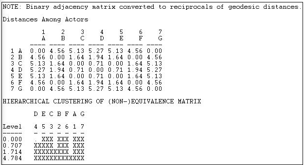
Figure 14.6: Automorphic equivalence of geodesic distances in the line network
The first step is to convert the adjacency matrix into a geodesic distance matrix. Then the reciprocal of the distance is taken, and a vector of the rows entries concatenated with the column entries for each actor is produced. The Euclidean distances between these lists are then created as a measure of the non-automorphic-equivalence, and hierarchical clustering is applied.
We see that actors 3 and 5 (C and E) form a class; actors 2 and 6 (B and F) form a class; actors 1 and 7 (A and G) form a class, and actor 4 (D) is a class. Mathematically, this is a sensible result; exchanges of labels of actors within these sets can occur and still produce an isomorphic distance matrix. The result also makes substantive sense -- and is quite like that for the Wasserman-Faust network.
This approximation method can also be applied where the data are valued. If we look at our data on donors to California political campaigns, we have measures of the strength of ties among the actors that are the number of positions in campaigns they have in common when either contributed. Figure 14.7 shows part of the output of Network>Roles & Positions>Automorphic>MaxSim.

Figure 14.7: Approximate automorphic equivalence of California political donors (truncated)
This small part of a large piece of output (there are 100 donors in the network) shows that a number of non-Indian casinos and race-tracks cluster together, and separately from some other donors who are primarily concerned with education and ecological issues.
The identification of approximate equivalence classes in valued data can be helpful in locating groups of actors who have a similar location in the structure of the graph as a whole. By emphasizing distance profiles, however, it is possible to finds classes of actors that include nodes that are quite distant from one another, but at a similar distance to all the other actors. That is, actors that have similar positions in the network as a whole.


