15.3: Finding Equivalence Sets
- Page ID
- 7742
\( \newcommand{\vecs}[1]{\overset { \scriptstyle \rightharpoonup} {\mathbf{#1}} } \)
\( \newcommand{\vecd}[1]{\overset{-\!-\!\rightharpoonup}{\vphantom{a}\smash {#1}}} \)
\( \newcommand{\id}{\mathrm{id}}\) \( \newcommand{\Span}{\mathrm{span}}\)
( \newcommand{\kernel}{\mathrm{null}\,}\) \( \newcommand{\range}{\mathrm{range}\,}\)
\( \newcommand{\RealPart}{\mathrm{Re}}\) \( \newcommand{\ImaginaryPart}{\mathrm{Im}}\)
\( \newcommand{\Argument}{\mathrm{Arg}}\) \( \newcommand{\norm}[1]{\| #1 \|}\)
\( \newcommand{\inner}[2]{\langle #1, #2 \rangle}\)
\( \newcommand{\Span}{\mathrm{span}}\)
\( \newcommand{\id}{\mathrm{id}}\)
\( \newcommand{\Span}{\mathrm{span}}\)
\( \newcommand{\kernel}{\mathrm{null}\,}\)
\( \newcommand{\range}{\mathrm{range}\,}\)
\( \newcommand{\RealPart}{\mathrm{Re}}\)
\( \newcommand{\ImaginaryPart}{\mathrm{Im}}\)
\( \newcommand{\Argument}{\mathrm{Arg}}\)
\( \newcommand{\norm}[1]{\| #1 \|}\)
\( \newcommand{\inner}[2]{\langle #1, #2 \rangle}\)
\( \newcommand{\Span}{\mathrm{span}}\) \( \newcommand{\AA}{\unicode[.8,0]{x212B}}\)
\( \newcommand{\vectorA}[1]{\vec{#1}} % arrow\)
\( \newcommand{\vectorAt}[1]{\vec{\text{#1}}} % arrow\)
\( \newcommand{\vectorB}[1]{\overset { \scriptstyle \rightharpoonup} {\mathbf{#1}} } \)
\( \newcommand{\vectorC}[1]{\textbf{#1}} \)
\( \newcommand{\vectorD}[1]{\overrightarrow{#1}} \)
\( \newcommand{\vectorDt}[1]{\overrightarrow{\text{#1}}} \)
\( \newcommand{\vectE}[1]{\overset{-\!-\!\rightharpoonup}{\vphantom{a}\smash{\mathbf {#1}}}} \)
\( \newcommand{\vecs}[1]{\overset { \scriptstyle \rightharpoonup} {\mathbf{#1}} } \)
\( \newcommand{\vecd}[1]{\overset{-\!-\!\rightharpoonup}{\vphantom{a}\smash {#1}}} \)
\(\newcommand{\avec}{\mathbf a}\) \(\newcommand{\bvec}{\mathbf b}\) \(\newcommand{\cvec}{\mathbf c}\) \(\newcommand{\dvec}{\mathbf d}\) \(\newcommand{\dtil}{\widetilde{\mathbf d}}\) \(\newcommand{\evec}{\mathbf e}\) \(\newcommand{\fvec}{\mathbf f}\) \(\newcommand{\nvec}{\mathbf n}\) \(\newcommand{\pvec}{\mathbf p}\) \(\newcommand{\qvec}{\mathbf q}\) \(\newcommand{\svec}{\mathbf s}\) \(\newcommand{\tvec}{\mathbf t}\) \(\newcommand{\uvec}{\mathbf u}\) \(\newcommand{\vvec}{\mathbf v}\) \(\newcommand{\wvec}{\mathbf w}\) \(\newcommand{\xvec}{\mathbf x}\) \(\newcommand{\yvec}{\mathbf y}\) \(\newcommand{\zvec}{\mathbf z}\) \(\newcommand{\rvec}{\mathbf r}\) \(\newcommand{\mvec}{\mathbf m}\) \(\newcommand{\zerovec}{\mathbf 0}\) \(\newcommand{\onevec}{\mathbf 1}\) \(\newcommand{\real}{\mathbb R}\) \(\newcommand{\twovec}[2]{\left[\begin{array}{r}#1 \\ #2 \end{array}\right]}\) \(\newcommand{\ctwovec}[2]{\left[\begin{array}{c}#1 \\ #2 \end{array}\right]}\) \(\newcommand{\threevec}[3]{\left[\begin{array}{r}#1 \\ #2 \\ #3 \end{array}\right]}\) \(\newcommand{\cthreevec}[3]{\left[\begin{array}{c}#1 \\ #2 \\ #3 \end{array}\right]}\) \(\newcommand{\fourvec}[4]{\left[\begin{array}{r}#1 \\ #2 \\ #3 \\ #4 \end{array}\right]}\) \(\newcommand{\cfourvec}[4]{\left[\begin{array}{c}#1 \\ #2 \\ #3 \\ #4 \end{array}\right]}\) \(\newcommand{\fivevec}[5]{\left[\begin{array}{r}#1 \\ #2 \\ #3 \\ #4 \\ #5 \\ \end{array}\right]}\) \(\newcommand{\cfivevec}[5]{\left[\begin{array}{c}#1 \\ #2 \\ #3 \\ #4 \\ #5 \\ \end{array}\right]}\) \(\newcommand{\mattwo}[4]{\left[\begin{array}{rr}#1 \amp #2 \\ #3 \amp #4 \\ \end{array}\right]}\) \(\newcommand{\laspan}[1]{\text{Span}\{#1\}}\) \(\newcommand{\bcal}{\cal B}\) \(\newcommand{\ccal}{\cal C}\) \(\newcommand{\scal}{\cal S}\) \(\newcommand{\wcal}{\cal W}\) \(\newcommand{\ecal}{\cal E}\) \(\newcommand{\coords}[2]{\left\{#1\right\}_{#2}}\) \(\newcommand{\gray}[1]{\color{gray}{#1}}\) \(\newcommand{\lgray}[1]{\color{lightgray}{#1}}\) \(\newcommand{\rank}{\operatorname{rank}}\) \(\newcommand{\row}{\text{Row}}\) \(\newcommand{\col}{\text{Col}}\) \(\renewcommand{\row}{\text{Row}}\) \(\newcommand{\nul}{\text{Nul}}\) \(\newcommand{\var}{\text{Var}}\) \(\newcommand{\corr}{\text{corr}}\) \(\newcommand{\len}[1]{\left|#1\right|}\) \(\newcommand{\bbar}{\overline{\bvec}}\) \(\newcommand{\bhat}{\widehat{\bvec}}\) \(\newcommand{\bperp}{\bvec^\perp}\) \(\newcommand{\xhat}{\widehat{\xvec}}\) \(\newcommand{\vhat}{\widehat{\vvec}}\) \(\newcommand{\uhat}{\widehat{\uvec}}\) \(\newcommand{\what}{\widehat{\wvec}}\) \(\newcommand{\Sighat}{\widehat{\Sigma}}\) \(\newcommand{\lt}{<}\) \(\newcommand{\gt}{>}\) \(\newcommand{\amp}{&}\) \(\definecolor{fillinmathshade}{gray}{0.9}\)The formal definition says that two actors are regularly equivalent if they have similar patterns of ties to equivalent others. Consider two men. Each has children (though they have different numbers of children, and, obviously have different children). Each has a wife (though again, usually different persons fill this role with respect to each man). Each wife, in turn, also has children and a husband (that is, they have ties with one or more members of each of those sets). Each child has ties to one or more members of the set of "husbands" and "wives".
In identifying which actors are "husbands" we do not care about ties between members of this set (actually, we would expect this block to be a zero block, but we really don't care). What is important is that each "husband" have at least one tie to a person in the "wife" category and at least one person in the "child" category. That is, husbands are equivalent to each other because each has similar ties to some member of the sets of wives and children.
But there would seem to be a problem with this fairly simple definition. If the definition of each position depends on its relations with other positions, where do we start?
There are a number of algorithms that are helpful in identifying regular equivalence sets. UCINET provides some methods that are particularly helpful for locating approximately regularly equivalent actors in valued, multi-relational and directed graphs. Some simpler methods for binary data can be illustrated directly.
Consider, again, the Wasserman-Faust example network. Imagine, however, that this is a picture of order-giving in a simple hierarchy. That is, all ties are directed from the top of the diagram in Figure 15.1 downward. We will find a regular equivalence characterization of this graph.
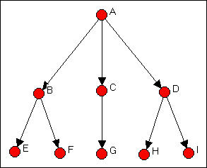
Figure 15.1: Directed tie version of the Wasserman-Faust network
For a first step, characterize each node as either a "source" (an actor that sends ties, but does not receive them), a "repeater" (an actor that both repeats and sends), or a "sink" (an actor that receives ties, but does not send them). The source is A; repeaters are B, C, and D; and sinks are E, F, G, H, and I. There is a fourth logical possibility. An "isolate" is a node that neither sends nor receives ties. Isolates form a regular equivalence set in any network, and should be excluded from the regular equivalence analysis of the connected sub-graph.
Since there is only one actor in the set of senders, we cannot identify any further complexity in this "role".
Consider the three "repeaters" B, C, and D. In the neighborhood of (that is, adjacent to) actor B are both "sources" and "sinks". The same is true for "repeaters" C and D, even though the three actors may have different numbers of sources and sinks, and these may be different (or the same) specific sources and sinks. We cannot define the "role" of the set {B, C, D} any further, because we have exhausted their neighborhoods. That is, the sources to whom our repeaters are connected cannot be further differentiated into multiple types (because there is only one source); the sinks to whom our repeaters send cannot be further differentiated, because they have no further connections themselves.
Now consider our "sinks" (i.e. actors E, F, G, H, and I). Each is connected to a source (although the sources may be different). We have already determined, in the current case, that all of these sources (actors B, C, and D) are regularly equivalent. So, E through I are equivalently connected to equivalent others. We are done with our partitioning.
The result of {A} {B, C, D} {E, F, G, H, I} satisfies the condition that each actor in each partition have the same pattern of connections to actors in other partitions. The permuted adjacency matrix is shown in Figure 15.2.

Figure 15.2: Permuted Wasserman-Faust network to show regular equivalence classes
It is useful to block this matrix and show its image. Here, however, we will use some special rules for determining zero and 1 blocks. If a block is all zeros, it will be a zero block. If each actor in a partition has a tie to any actor in another, then we will define the joint block as a 1-block. Bear with me a moment. The image using this rule is shown in Figure 15.3.

Figure 15.3: Block image of regular equivalence classes in directed Wasserman-Faust network
{A} sends to one or more of {BCD} but to none of {EFGHI}. {BCD} does not send to {A}, but each of {BCD} sends to at least one of {EFGHI}. None of {EFGHI} send to any of {A}, or of {BCD}. The image, in fact, displays the characteristic pattern of a strict hierarchy: ones on the first off-diagonal vector and zeros elsewhere. The rule of defining a 1-block when each actor in one partition has a relationship with any actor in the other partition is a way of operationalizing the notion that the actors in the first set are equivalent if they are connected to equivalent actors (i.e. actors in the other partition), without requiring (or prohibiting) that they be tied to the same other actors, or the same number of actors in another partition.
For directed binary graphs, the neighborhood search method we applied here usually works quite well. For binary graphs that are not directed, usually the geodesic distance among actors is computed and used instead of raw adjacency. For graphs with valued relations (strength, cost, probability), a method for identifying approximate regular equivalence was developed by White and Reitz. These several alternatives are illustrated below.
Categorical REGE for Directed Binary Data (Wasserman-Faust Directed Network)
The neighborhood search method illustrated above (with the directed Wasserman-Faust network) is the algorithm performed by Network>Roles & Positions>Maximal Regular>CATREGE. This approach is ideal for networks where relations are measured at the nominal level, and are directed. Our example will be of a binary graph; the algorithm, however, can also deal with multi-valued nominal data (e.g. "1" = friend, "2" = kin, "3" = coworker, etc.).
Applying Network>Roles & Positions>Maximal Regular>CATREGE to the Wasserman-Faust directed network gives the results shown in Figure 15.4.
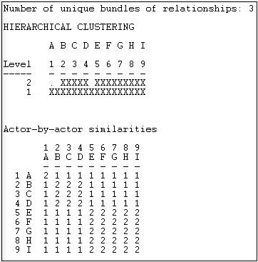
Figure 15.4: Categorical REGE analysis of Wasserman-Faust directed network
This result is the same as the one that we did "by hand" earlier in the chapter. A hierarchical clustering diagram can be useful if the equivalences found are inexact, or numerous, and a further simplification is needed. Here, we see at level 2 of the clustering that there are three groups {A}, {B, C, D}, and {E, F, G, H, I}. An image matrix is also produced (but not "reduced" to 3 by 3).
The results can also be usefully visualized with a dendogram, as in Figure 15.5.
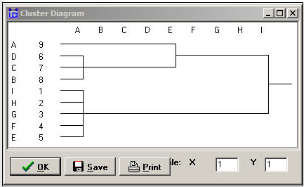
Figure 15.5: Dendogram of categorical REGE (Figure 15.4)
We know, from our analysis, that there really are exactly three regular equivalence classes. Should we want to use only two, however, the dendogram suggests that grouping A with B, C, and D would be the most reasonable choice.
Once a regular equivalence blocking has been achieved, it is usually a good idea to produce a permuted and blocked version of the original data so that you can see the tie profiles of each of the classes. One way to do this is to save the permutation vector from Network>Roles & Positions>Maximal Regular>CATREGE, and use it to permute the original data (Data>Permute).
Categorical REGE for Geodesic Distances (Padgett's Marriage Data)
The Padgett data on marriage alliances among leading Florentine families are of low to moderate density. There are considerable differences among the positions of the families, as can be seen from the graph in Figure 15.6. The data are binary, and not directed. This causes a problem for regular equivalence analysis, because all actors (except isolates) are "equivalent" as "transmitters".
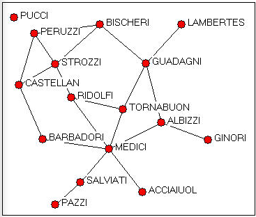
Figure 15.6: Padgett Florentine marriage alliances
The categorical REGE algorithm (Network>Roles & Positions>Maximal Regular>CATREGE) can be used to identify regularly equivalent actors by treating the elements of the geodesic distance matrix as describing "types" of ties - that is different geodesic distances are treated as "qualitatively" rather than "quantitatively" different. Two nodes are more equivalent if each has an actor in their neighborhood of the same "type". In this case, that means they are similar if they each have an actor that is at the same geodesic distance from themselves. With many data sets, the levels of similarity of neighborhoods can turn out to be quite high - and it may be difficult to differentiate the positions of the actors on "regular" equivalence grounds.
Figure 15.7 shows the results of regular equivalence analysis where geodesic distances have been used to represent multiple qualitative types of relations among actors.
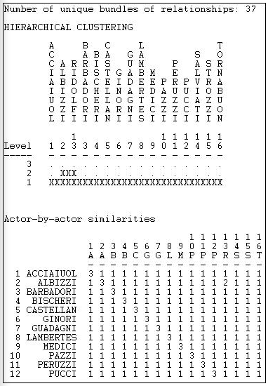
Figure 15.7: Categorical multi-value analysis (geodesic distance) of Padgett marriage alliances
Since the data are highly connected and geodesic distances are short, we are not able to discriminate highly distinctive regular classes in these data. Two families (Albizzi and Ridolfi) do emerge as more similar than others, but generally the differences among profiles is small.
The use of REGE with undirected data, even substituting geodesic distances for binary values, can produce rather unexpected results. It may be more useful to combine a number of different ties to produce continuous values. The main problem, however, is that with undirected data, most cases will appear to be very similar to one another (in the "regular" sense), and no algorithm can really "fix" this. If geodesic distances can be used to represent differences in the types of ties (and this is a conceptual question), and if the actors do have some variability in their distances, this method can produce meaningful results. But, in my opinion, it should be used cautiously, if at all, with undirected data.
Continuous REGE for Geodesic Distances (Padgett's Marriage Data)
An alternative approach to the undirected Padgett data is to treat the different levels of geodesic distances as measures of (the inverse of) strength of ties. Two nodes are said to be more equivalent if they have an actor of similar distance in their neighborhood (similar in the quantitative sense of "5" is more similar to "4" than "6" is). By default, the algorithm extends the search to neighborhoods of distance 3 (though less or more can be selected).
Figure 15.8 shows the results of applying Network>Roles & Positions>Maximal Regular>REGE to the Padgett data, using "3 iterations" (that is, three-step neighborhoods).
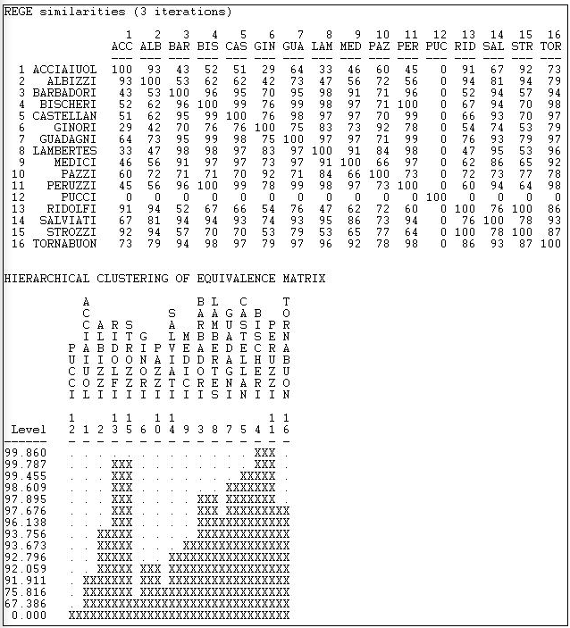
Figure 15.8: Continuous REGE of Padgett marriage alliance data
The first panel of the output displays the approximate pair-wise regular similarities as a matrix. Note that the isolated family (Pucci) is treated as a separate class. Also note that these results are finding rather different features of the data than did the categorical treatment. The continuous REGE algorithm applied to the undirected data is probably a better choice than the categorical approach. The result still shows very high regular equivalence among the actors, and the solution is only modestly similar to that of the categorical approach.
The Knoke Bureaucracies Information Exchange Network Analyzed by Tabu Search
At the end of our analysis in the section "Finding Equivalence Sets" above, we produced a "permuted and blocked" version of our data. In doing this, we used a few rules that, in fact, identify what regular equivalence relations "look like". To repeat the main points: we don't care about the ties among members of a regular class; ties between members of a regular class and another class are either all zero, or such that each member of one class has a tie to at least one member of the other class.
This "picture" of what regular classes look like can be used to search for them using numerical methods. The Network>Roles & Positions>Maximal Regular>Optimization algorithm seeks to sort nodes into (a user selected number of) categories that come as close to satisfying the "image" of regular equivalence as possible. Figure 15.9 shows the results of applying this algorithm to the Knoke information network.
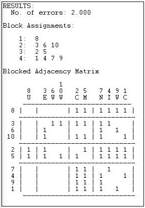
Figure 15.9: Four regular equivalence classes for the Knoke information network by optimum search
The method produces a fit statistic (number of errors), and solutions for different numbers of partitions should be compared.
The blocked adjacency matrix for the four group solution is, however, quite convincing. Of the 12 block of interest (the blocks on the diagonal are not usually treated as relevant to "role" analysis) 11 satisfy the rules for zero or one blocks perfectly. Only the block connecting sending from {3, 6, 10} to the block {2, 5} fails to satisfy the image of regular equivalence (because actor 6 has no sending ties to either actor 2 or 5).
The solution is also an interesting one substantively. The third set {2, 5} for example, are pure "repeaters" sending and receiving from all other roles. The set {3, 6, 10} send to only two other types (not all three other types) and receive from only one other type. And so on.
The tabu search method can be very useful, and usually produces quite nice results. It is an iterative search algorithm, however, and can find local solutions. Many networks have more than one valid partitioning by regular equivalence, and there is no guarantee that the algorithm will always find the same solution. It should be run a number of times with different starting configurations.


