
18.3: Synchronizability


- Last updated
- Apr 30, 2024
- Save as PDF

( \newcommand{\kernel}{\mathrm{null}\,}\)
An interesting application of the spectral gap/algebraic connectivity is to determine the synchronizability of linearly coupled dynamical nodes, which can be formulated as follows:
dxidt=R(xi)+α∑jϵNi(H(xj)−H(xi))
Here xi is the state of node i, R is the local reaction term that produces the inherent dynamica lbehavior of individual nodes, and Ni is the neighborhood of node i. We assume that R is identical for all nodes, and it produces a particular trajectory xs(t) if there is no interaction with other nodes. Namely, xs(t) is given as the solution of the differential equation dx/dt=R(x). H is called the output function that homogeneously applies to all nodes. The output function is used to generalize interaction and diffusion among nodes; instead of assuming that the node states themselves are directly visible to others, we assume that a certain aspect of node states (represented by H(x)) is visible and diffusing to other nodes.
Equation ??? can be further simplified by using the Laplacian matrix, as follows:
dxidt=R(xi)−αL(H(x1)H(x2)⋮H(xn))
Now we want to study whether this network of coupled dynamical nodes can synchronize or not. Synchronization is possible if and only if the trajectory xi(t)=xs(t) for all i is stable. This is a new concept, i.e., to study the stability of a dynamic trajectory, not of a static equilibrium state. But we can still adopt the same basic procedure of linear stability analysis: represent the system’s state as the sum of the target state and a small perturbation, and then check if the perturbation grows or shrinks over time. Here we represent the state of each node as follows:
xi(t)=xs(t)+Δxi(t)
By plugging this new expression into Equation ???, we obtain
d(xs+Δxi)dt=R(xs+Δxi)−αL(H(xs+Δx1)H(xs+Δx2)⋮H(xs+Δxn))
Since ∆xi are very small, we can linearly approximate R and H as follows:
dxsdt+dΔxidt=R(xs)+R′(xs)Δxi−αL(H(xs)+H′(xs)Δx1H(xs)+H′(xs)Δx2⋮H(xs)+H′(xs)Δxn)
The first terms on both sides cancel out each other because xs is the solution of dx/dt=R(x) by definition. But what about those annoying H(xs)’s included in the vector in the last term? Is there any way to eliminate them? Well, the answer is that we don’t have to do anything, because the Laplacian matrix will eat them all. Remember that a Laplacian matrix always satisfies Lh=0. In this case, those H(xs)’s constitute a homogeneous vector H(xs)h altogether. Therefore,L(H(xs)h)=H(xs)Lh vanishes immediately, and we obtain
dΔxdt=R′(xs)Δxi−αH′(xs)L(Δx1Δx2⋮Δxn),
or, by collecting all the ∆xi’s into a new perturbation vector ∆x,
dΔxdt=(R′(xs)I−αH′(xs)L)Δx,
as the final result of linearization. Note that xs still changes over time, so in order for this trajectory to be stable, all the eigenvalues of this rather complicated coefficient matrix (R'(x_s)I −αH'(x_s)L) should always indicate stability at any point in time.
We can go even further. It is known that the eigenvalues of a matrix aX+bI are aλ_i+b, where λ_i are the eigenvalues of X. So, the eigenvalues of (R'(x_s)I −αH'(x_s)L are
-\alpha{\lambda_{i}}H'(x_s) +R'(x_s), \label{(18.13)}
where λ_i are L’sneigenvalues. The eigenvalue that corresponds to the smallest eigenvalue of L, 0, is just R'(x_s), which is determined solely by the inherent dynamics of R(x) (and thus the nature of x_s(t)), so we can’t do anything about that. But all the other n − 1 eigenvalues must be negative all the time, in order for the target trajectory x_s(t) to be stable. So, if we represent the second smallest eigenvalue (the spectral gap for connected networks) and the largest eigenvalue of L by λ_{2} and λ_n, respectively, then the stability criteria can be written as
\alpha{\lambda_{i}}H'(x_{s}(t)) >R' (x_{s}(t)) \qquad{\text{for all t, and}} \label{(18.14)}
\alpha{\lambda_n}H'(x_s(t)) >R'(x_s(t)) \qquad{\text{ for all t, }} \label{(18.15)}
because all other intermediate eigenvalues are “sandwiched” by λ_2 and λ_n. These inequalities provide us with a nice intuitive interpretation of the stability condition: the influence of diffusion of node outputs (left hand side) should be stronger than the internal dynamical drive (right hand side) all the time.
Note that, although α and λ_i are both non-negative, H'(xs(t)) could be either positive or negative, so which inequality is more important depends on the nature of the output function H and the trajectory x_s(t) (which is determined by the reaction term R). If H'(x_s(t)) always stays non-negative, then the first inequality is sufficient (since the second inequality naturally follows as λ_2 ≤ λ_n), and thus the spectral gap is the only relevant information to determine the synchronizability of the network. But if not, we need to consider both the spectral gap and the largest eigenvalue of the Laplacian matrix.
Here is a simple example. Assume that a bunch of nodes are oscillating in an exponentially accelerating pace:
\frac{d\theta_i}{dt} =\beta{\theta_i} +\alpha \sum_{j \epsilon{N_i} (\theta_{j} - \theta_{i})} \label{(18.16)}
Here, θ_i is the phase of node i, and β is the rate of exponential acceleration that homogeneously applies to all nodes. We also assume that the actual values of θi diffuse to and from neighbor nodes through edges. Therefore, R(θ) = βθ and H(θ) = θ in this model.
We can analyze the synchronizability of this model as follows. Since H'(θ) = 1 > 0, we immediately know that the inequality \ref{(18.14)} is the only requirement in this case. Also, R'(θ) = β, so the condition for synchronization is given by
\alpha{\lambda_2} > \beta, \text{or} \lambda_2 > \frac{\beta}{\alpha}. \label{(18.17)}
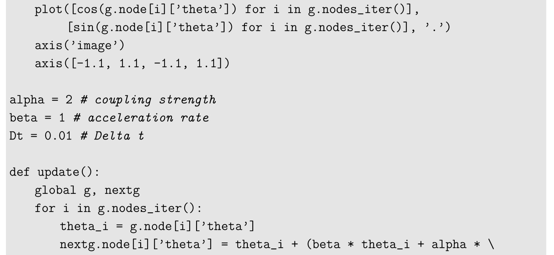
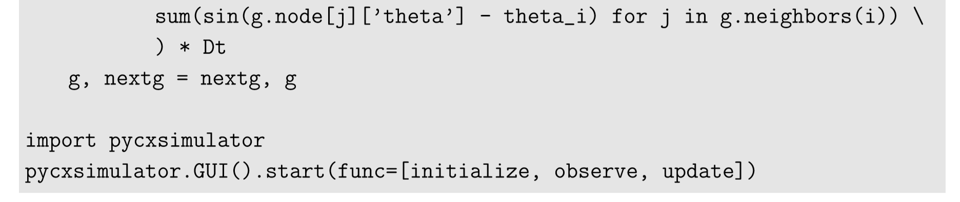
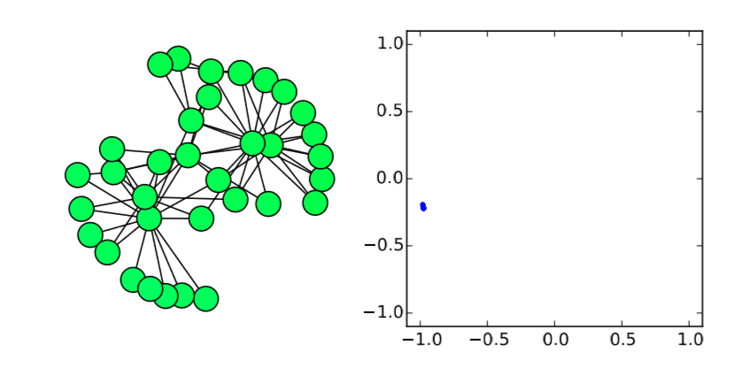
Very easy. Let’s check this analytical result with numerical simulations on the Karate Club graph. We know that its spectral gap is 0.4685, so if β/α is below (or above) this value, the synchronization should (or should not) occur. Here is the code for such simulations:

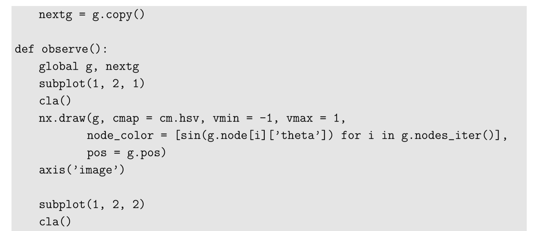
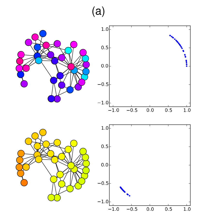
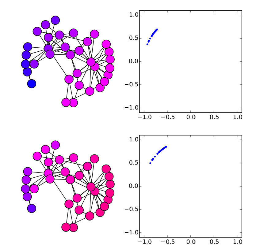
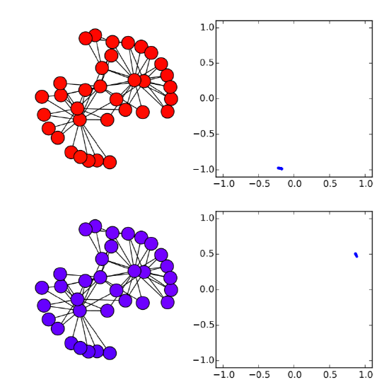
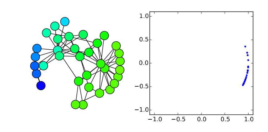
Here I added a second plot that shows the phase distribution in a (x,y) = (cos{θ},sin{θ}) space, just to aid visual understanding.
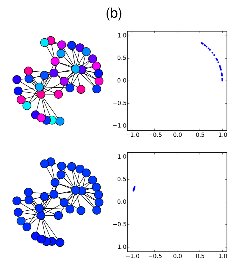
In the code above, the parameter values are set to alpha = 2 and beta = 1, so λ_2 0.4685 < β/α = 0.5. Therefore, it is predicted that the nodes won’t get synchronized. And, indeed, the simulation result confirms this prediction (Fig. 18.3.1(a)), where the nodes initially came close to each other in their phases but, as their oscillation speed became faster and faster, they eventually got dispersed again and the network failed to achieve synchronization. However, if beta is slightly lowered to 0.9 so that λ_2 = 0.4685 > β/α = 0.45, the synchronized state becomes stable, which is confirmed again in the numerical simulation (Fig. 18.3.1(b)). It is interesting that such a slight change in the parameter value can cause a major difference in the global dynamics of the network. Also, it is rather surprising that the linear stability analysis can predict this shift so precisely. Mathematical analysis rocks!
Randomize the topology of the Karate Club graph and measure its spectral gap. Analytically determine the synchronizability of the accelerating oscillators model discussed above with α = 2, β = 1 on the randomized network. Then confirm your prediction by numerical simulations. You can also try several other network topologies.
he following is a model of coupled harmonic oscillators where complex node states are used to represent harmonic oscillation in a single-variable differential equation:
\frac{dx_i}{dt} =i\omega{x_i} +\alpha \sum{j\epsilon{N_i}(x^{\gamma}_{j} -x^{y}_{i})} \label{(18.18)}
Here i is used to denote the imaginary unit to avoid confusion with node index i. Since the states are complex, you will need to use Re(·) on both sides of the inequalities \ref{(18.14)} and \ref{(18.15)} to determine the stability.
Analyze the synchnonizability of this model on the Karate Club graph, and obtain the condition for synchronization regarding the output exponent γ. Then confirm your prediction by numerical simulations.
You may have noticed the synchronizability analysis discussed above is somewhat similar to the stability analysis of the continuous field models discussed in Chapter 14. Indeed, they are essentially the same analytical technique (although we didn’t cover stability analysis of dynamic trajectories back then). The only difference is whether the space is represented as a continuous field or as a discrete network. For the former, the diffusion

is represented by the Laplacian operator ∇^2, while for the latter, it is represented by the Laplacian matrix L (note again that their signs are opposite for historical misfortune!). Network models allows us to study more complicated, nontrivial spatial structures, but there aren’t any fundamentally different aspects between these two modeling frameworks. This is why the same analytical approach works for both.
Note that the synchronizability analysis we covered in this section is still quite limited in its applicability to more complex dynamical network models. It relies on the assumption that dynamical nodes are homogeneous and that they are linearly coupled, so the analysis can’t generalize to the behaviors of heterogeneous dynamical networks with nonlinear couplings, such as the Kuramoto model discussed in Section 16.2 in which nodes oscillate in different frequencies and their couplings are nonlinear. Analysis of such networks will need more advanced nonlinear analytical techniques, which is beyond the scope of this textbook.