4.4: Simulating Discrete-Time Models with Multiple Variables

Now we are making a first step to complex systems simulation. Let’s increase the number of variables from one to two. Consider the following difference equations:

\[x_{t} =0.5_{t-1} +y_{t-1}\label{4.14)} \]

\[y_{t}=-0.5x_{t-1} +y_{t-1}\label{(4.15)} \]

with

\[x_{0} =1, y_{0}=1\label{(4.16)} \]

These equations can also be written using vectors and a matrix as follows:

\[\binom{x}{y} =\binom{0.5 \ \ 1}{-0.5 \ \ 1} \binom{x}{y}_{t-1}\label{(4.17)} \]

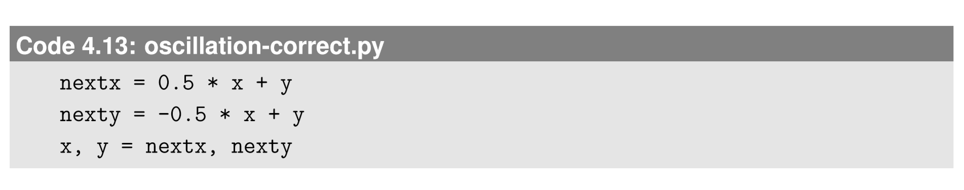
Try implementing the simulation code of the equation above. This may seem fairly straightforward, requiring only minor changes to what we had before. Namely, you just need to simulate two difference equations simultaneously. Your new code may look like this:

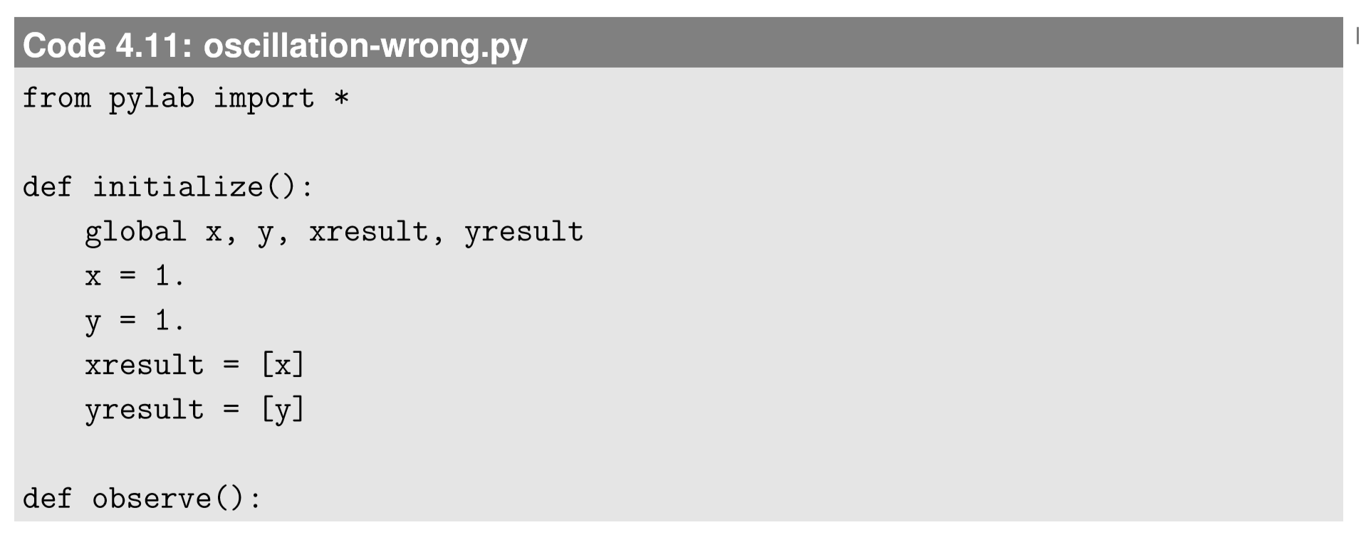
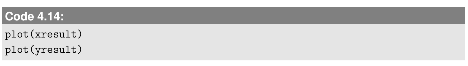
What I did in this code is essentially to repeat things for both x and y. Executing two plot commands at the end produces two curves in a single chart. I added the ’b-’ and ’g--’ options to the plot functions to draw xresult in a blue solid curve and y result in a green dashed curve. If you run this code, it produces a decent result (Fig. 4.4.1), so things might look okay. However, there is one critical mistake I made in the code above. Can you spot it? This is a rather fundamental issue in complex systems simulation in general, so we’d better notice and fix it earlier than later. Read the code carefully again, and try to find where and how I did it wrong.

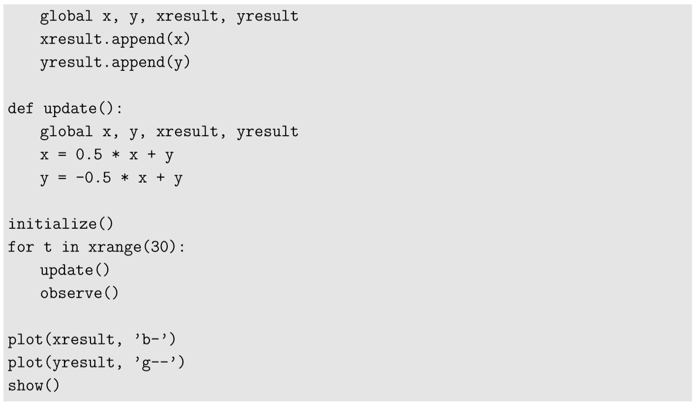
Did you find it? The answer is that I did not do a good job in updating x and y simultaneously. Look at the following part of the code:

Note that, as soon as the first line is executed, the value of x is overwritten by its new value. When the second line is executed, the value of x on its right hand side is already updated,but it should still be the original value. In order to correctly simulate simultaneous updating of x and y, you will need to do something like this:

Figure \(\PageIndex{1}\): Visual output of Code 4.11. This result is actually wrong.

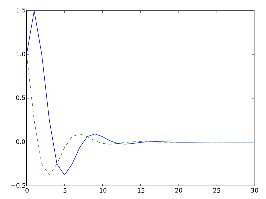
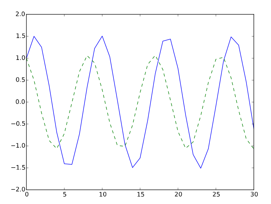
Here we have two sets of state variables, x, y and nextx, nexty. We first calculate the next state values and store them in nextx, nexty, and then copy them to x, y, which will be used in the next iteration. In this way, we can avoid any interference between the state variables during the updating process. If you apply this change to the code, you will get a correct simulation result (Fig. 4.4.2).

The issue of how to implement simultaneous updating of multiple variables is a common technical theme that appears in many complex systems simulation models, as we will discuss more in later chapters. As seen in the example above, a simple solution is to prepare two separate sets of the state variables, one for now and the other for the immediate future, and calculate the updated values of state variables without directly modifying them during the updating. In the visualizations above, we simply plotted the state variables over time, but there is

Figure \(\PageIndex{2}\): Visual output of the simulation result based on a correctly implemented code with Code 4.13.

another way of visualizing simulation results in a phase space. If your model involves just two state variables (or three if you know 3-D plotting), you should try this visualization to see the structure of the phase space. All you need to do is to replace the following part

with this:

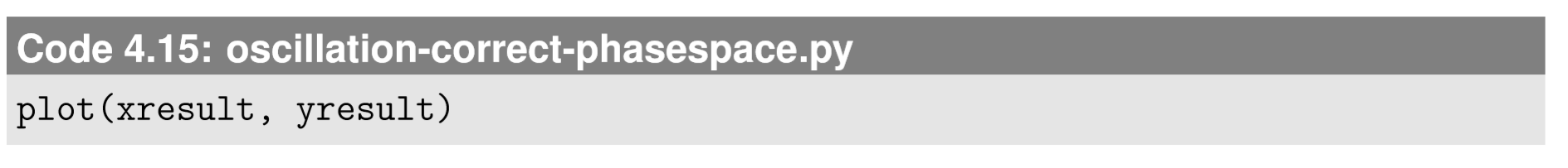
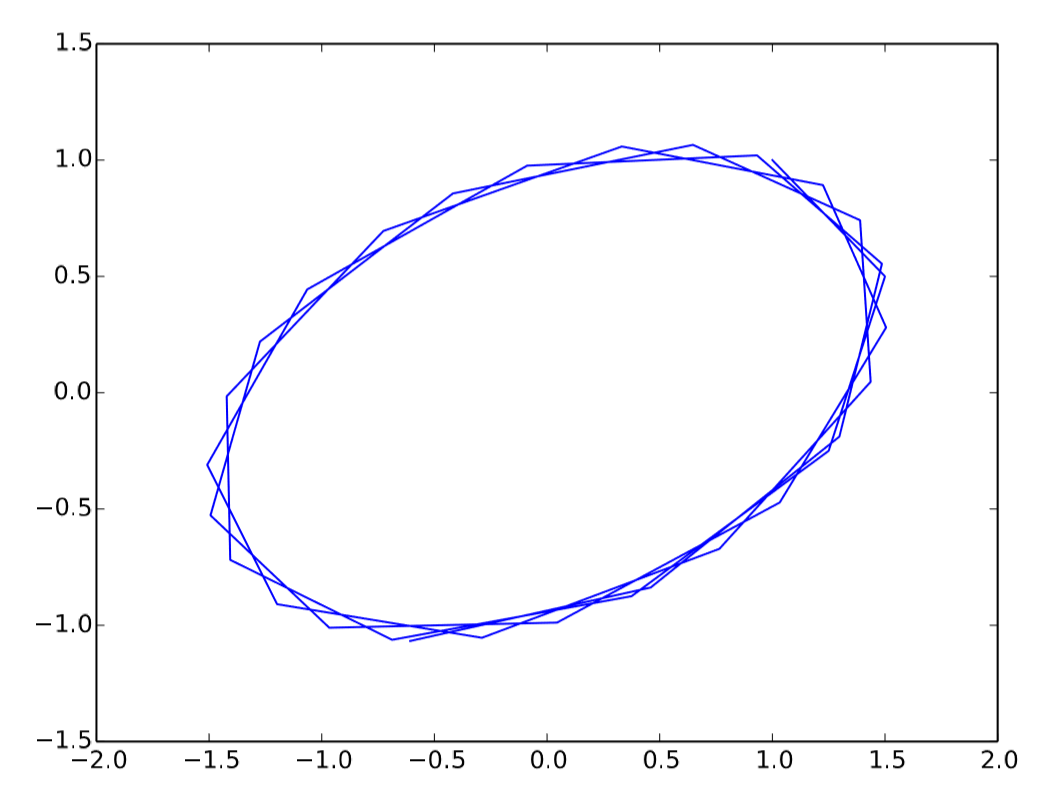
This will produce a trajectory of the system state in an \(x-y\) phase space, which clearly shows that the system is in an oval, periodic oscillation (Fig. 4.4.3), which is a typical signature of a linear system.

Figure \(\PageIndex{3}\): Visualization of the simulation result in a phase space using Code 4.15.

Exercise \(\PageIndex{1}\)

Simulate the above two-variable system using several different co-efficients in the equations and see what kind of behaviors can arise.

Exercise \(\PageIndex{2}\)

Simulate the behavior of the following Fibonacci sequence. You first need to convert it into a two-variable first-order difference equation, and then implement a simulation code for it.

\[x_{t} = x_{t-1} +x_{t-2}, x_{0} =1, x_{1}=1\label{(4.18)} \]

If you play with this simulation model for various coefficient values, you will soon notice that there are only certain kinds of behaviors possible in this system. Sometimes the curves show exponential growth or decay, or sometimes they show more smooth oscillatory behaviors. These two behaviors are often combined to show an exponentially growing oscillation, etc. But that’s about it. You don’t see any more complex behaviors coming out of this model. This is because the system is linear, i.e., the model equation is composed of a simple linear sum of first-order terms of state variables. So here is an important fact you should keep in mind:

Linear dynamical systems can show only exponential growth/decay, periodic oscillation, stationary states (no change), or their hybrids (e.g., exponentially growing oscillation)^a.

^aSometimes they can also show behaviors that are represented by polynomials (or products of polynomials and exponentials) of time. This occurs when their coefficient matrices are non-diagonalizable.

In other words, these behaviors are signatures of linear systems. If you observe such behavior in nature, you may be able to assume that the underlying rules that produced the behavior could be linear.