8.4: Bifurcations in Discrete-Time Models
( \newcommand{\kernel}{\mathrm{null}\,}\)
The bifurcations discussed above (saddle-node, transcritical, pitchfork, Hopf) are also possible in discrete-time dynamical systems with one variable:
xt=F(xt−1)
The Jacobian matrix of this system is, again, a 1×1 matrix whose eigenvalue is its content itself, which is given by dF/dx. Since this is a discrete-time model, the critical condition at which a bifurcation occurs is given by
|dFdt|x=xeq=1.
Let’s work on the following example:
xt=xt−1+r−x2t−1
This is a discrete-time analog of Eq. (8.1.3). Therefore, it has the same set of equilibrium points:
xeq=±√r
Next, we calculate dF/dx as follows:
dFdx=(r+x−x2)′=1−2x|dFdt|x=±√r=|1±2√r|
To find out which value of r makes this 1, we consider the following four scenarios:
- 1+2√r=1⇒r=0
- 1−2√r=1⇒r=0
- 1+2√r=−1⇒(no real solution)
- 1−2√r=−1⇒r=1
As you see, r=0 appears as a critical threshold again, at which a saddle-node bifurcation occurs. But now we see another critical threshold, r=1, also showing up, which was not there in its continuous-time version. This is why I said before that continuous-time models are simpler than discrete-time \ models for bifurcation analysis; discrete-time models can show a new form of bifurcation that wasn’t possible in their continuous-time counterparts. To learn more about this, we can study the stability of the two equilibrium points by checking whether |dF/dx| is greater or less than 1 at each point. The result is summarized in Table 8.4.1.
Table 8.4.1: Summary of bifurcation analysis of xt=xt−1+r−x2t−1.
| Equilibrium point | r<0 | 0<r<1 | 1<r |
|---|---|---|---|
| xeq=√r | doesn’t exist | stable | unstable |
| xeq=−√r | doesn’t exist | unstable | unstable |
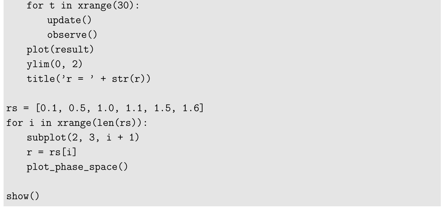
The result shown in the table is pretty much the same as before up to r=1, but when r>1, both equilibrium points become unstable. This must mean that the system is not allowed to converge toward either of them. Then what is going to happen to the system in this parameter range? We can let the system show its actual behavior by numerical simulations. Here is an example:


The results are shown in Fig. 8.4.1, visualizing actual trajectories of the system’s state over time for several values of r. The cobweb plot version is also shown in Fig. 8.4.2 (the code is not shown here; try implementing the code yourself!).
There are some new behaviors that were not seen in continuous-time versions of the same model. For example, at r=0.5, there was a signature of “overshooting” right before the system state converged to a stable equilibrium point. But more importantly, at r=1, the system began to fail to converge to a single stable point, and for r>1, it started oscillating between two distinct states. This is called a period−doubling bifurcation. It is a bifurcation that typically occurs in discrete-time systems (but it is also possible in continuous-time systems of higher dimensions), where the system loses stability of a period T trajectory and begins to move in another trajectory with period 2T. The bifurcation observed for r=1 was a transition from an equilibrium point (which is a periodic trajectory with period T=1, i.e., the system takes the same state value in each time step)
to a trajectory with period 2T=2. Interestingly, the period-doubling bifurcations happen in a cascade if you keep increasing r. In this particular case, another period-doubling bifurcation was observed at r=1.5, where the period-2 trajectory lost its stability and the system moved to a period-4 trajectory. This continues as you continue to increase r. The first period-doubling bifurcation from period-1 to period-2 trajectories can still be characterized as the loss of stability of an equilibrium point, but the dominant eigenvalue destabilizing the equilibrium point must be negative in order to induce the flipping behavior. This can be mathematically written as follows:
A first period-doubling bifurcation from period-1 to period-2 trajectories occurs in a discrete-time model when the eigenvalues λi of the Jacobian matrix at an equilibrium point satisfy the following:
λi=−1 for some i, while|λi|<1 for the rest.
In the example above, dF/dx|xeq=√r=−1 when r=1, which triggers the first period doubling bifurcation.
Consider the following discrete-time dynamical system:
xt=(1−a)xt−1+ax3t−1
This equation has xeq=0 as an equilibrium point. Obtain the value of a at which this equilibrium point undergoes a first period-doubling bifurcation.
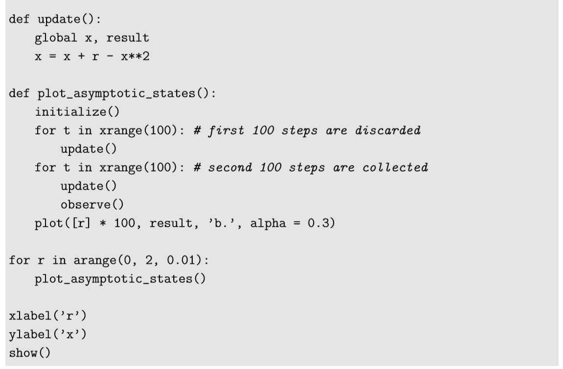
Once the system begins to show period-doubling bifurcations, its asymptotic states are no longer captured by the locations of analytically obtained equilibrium points, as drawn in bifurcation diagrams (e.g., Figs. 8.2.1, 8.2.3, etc.). However, there is still a way to visualize bifurcation diagrams numerically by simulating the behavior of the system explicitly and then collecting the actual states the system visits for a certain period of time. Then we can plot their distributions in a diagram. The data points should be collected after a sufficiently long initial transient time has passed in each simulation, so that the system’s trajectory is already showing its “final” behavior. Here is a sample code showing how to draw such a bifurcation diagram numerically:


In this code, r is gradually varied from 0 to 2 at intervals of 0.01. For each value of r, the model (Equation ???) is simulated for 200 steps, and only the second half of the state values are recorded in result. Once the simulation is finished, the states stored in result are plotted at a particular value of r in the plot (note that the expression [r] * 100 in Python produces a list of one hundred r’s). The alpha option is used to make the markers transparent so that the densities of markers are also visible.
The result is shown in Fig. 8.4.3. This bifurcation diagram still shows how the system’s state depends on the parameter, but what is plotted here are no longer analytically obtained equilibrium points but numerically sampled sets of asymptotic states, i.e., where the system is likely to be after a sufficiently long period of time. If the system is converging to a stable equilibrium point, you see one curve in this diagram too. Unstable equilibrium points never show up because they are never realized in numerical simulations. Once the system undergoes period-doubling bifurcations, the states in a periodic trajectory are all sampled during the sampling period, so they all appear in this diagram. The period doubling bifurcations are visually seen as the branching points of those curves.
But what are those noisy, crowded, random-looking parts at r>1.7? That is chaos, the hallmark of nonlinear dynamics. We will discuss what is going on there in the next chapter.
Period-doubling bifurcations and chaos are not just for abstract, contrived mathematical equations, but they can occur in various models of real-world biological, ecological, social, and engineering phenomena. The simplest possible example would be the logistic map we introduced in Section 5.5:
xt=rxt−1(1−xt−1)
This is a mathematical model of population dynamics, where xt represents the population of a species that reproduce in discrete (non-overlapping) generations. This model was used by British/Australian mathematical ecologist Robert May in his influential 1976 Nature paper [32] to illustrate how a very simple mathematical model could produce astonishingly complex behaviors.
- Conduct a bifurcation analysis of this model to find the critical thresholds of r at which bifurcations occur.
- Study the stability of each equilibrium point in each parameter range and summarize the results in a table.
- Simulate the model with several selected values of r to confirm the results of analysis.
- Draw a bifurcation diagram of this model for 0<r<4.
The stability of a period-2 trajectory of a discrete-time model xt=F(xt−1) can be studied by the stability analysis of another model made of a composite function of F:
yr=G(yτ−1)=F(F(tτ−1))
This is because the period-2 trajectory in F corresponds to one of the equilibrium points of G(◦) = F(F(◦)). If such an equilibrium point of G is being destabilized so that dG/dx ≈−1, it means that the period-2 trajectory in question is losing the stability, and thus another period-doubling bifurcation into a period-4 trajectory is about to occur. Using this technique, analytically obtain the critical threshold of r in Equation \ref{(8.37)} at which the second period-doubling bifurcation occurs (from period 2 to period 4). Then, draw cobweb plots of y_τ = G(y_{τ−1}) for several values of r near the critical threshold to see what is happening there.


