
15.5: Importing/Exporting Network Data
- Page ID
- 7861

\( \newcommand{\vecs}[1]{\overset { \scriptstyle \rightharpoonup} {\mathbf{#1}} } \)
\( \newcommand{\vecd}[1]{\overset{-\!-\!\rightharpoonup}{\vphantom{a}\smash {#1}}} \)
\( \newcommand{\id}{\mathrm{id}}\) \( \newcommand{\Span}{\mathrm{span}}\)
( \newcommand{\kernel}{\mathrm{null}\,}\) \( \newcommand{\range}{\mathrm{range}\,}\)
\( \newcommand{\RealPart}{\mathrm{Re}}\) \( \newcommand{\ImaginaryPart}{\mathrm{Im}}\)
\( \newcommand{\Argument}{\mathrm{Arg}}\) \( \newcommand{\norm}[1]{\| #1 \|}\)
\( \newcommand{\inner}[2]{\langle #1, #2 \rangle}\)
\( \newcommand{\Span}{\mathrm{span}}\)
\( \newcommand{\id}{\mathrm{id}}\)
\( \newcommand{\Span}{\mathrm{span}}\)
\( \newcommand{\kernel}{\mathrm{null}\,}\)
\( \newcommand{\range}{\mathrm{range}\,}\)
\( \newcommand{\RealPart}{\mathrm{Re}}\)
\( \newcommand{\ImaginaryPart}{\mathrm{Im}}\)
\( \newcommand{\Argument}{\mathrm{Arg}}\)
\( \newcommand{\norm}[1]{\| #1 \|}\)
\( \newcommand{\inner}[2]{\langle #1, #2 \rangle}\)
\( \newcommand{\Span}{\mathrm{span}}\) \( \newcommand{\AA}{\unicode[.8,0]{x212B}}\)
\( \newcommand{\vectorA}[1]{\vec{#1}} % arrow\)
\( \newcommand{\vectorAt}[1]{\vec{\text{#1}}} % arrow\)
\( \newcommand{\vectorB}[1]{\overset { \scriptstyle \rightharpoonup} {\mathbf{#1}} } \)
\( \newcommand{\vectorC}[1]{\textbf{#1}} \)
\( \newcommand{\vectorD}[1]{\overrightarrow{#1}} \)
\( \newcommand{\vectorDt}[1]{\overrightarrow{\text{#1}}} \)
\( \newcommand{\vectE}[1]{\overset{-\!-\!\rightharpoonup}{\vphantom{a}\smash{\mathbf {#1}}}} \)
\( \newcommand{\vecs}[1]{\overset { \scriptstyle \rightharpoonup} {\mathbf{#1}} } \)
\( \newcommand{\vecd}[1]{\overset{-\!-\!\rightharpoonup}{\vphantom{a}\smash {#1}}} \)
In most network studies, researchers need to model and analyze networks that exist in the real world. To do so, we need to learn how to import (and export) network data from outside Python/NetworkX. Fortunately, NetworkX can read and write network data from/to files in a number of formats2.
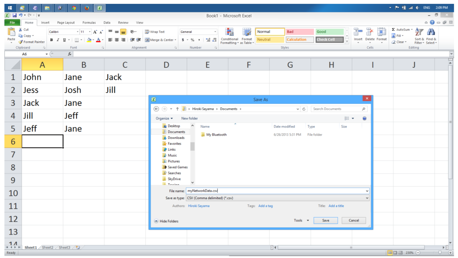
off’) right after the network drawing.Let’s work on a simple example. You can create your own adjacency list in a regular spreadsheet (such as Microsoft Excel or Google Spreadsheet) and then save it in a “csv” format file (Fig. 15.5.2). In this example, the adjacency list says that John is connected to Jane and Jack; Jess is connected to Josh and Jill; and so on.
You can read this file by using the read_adjlist command, as follows:
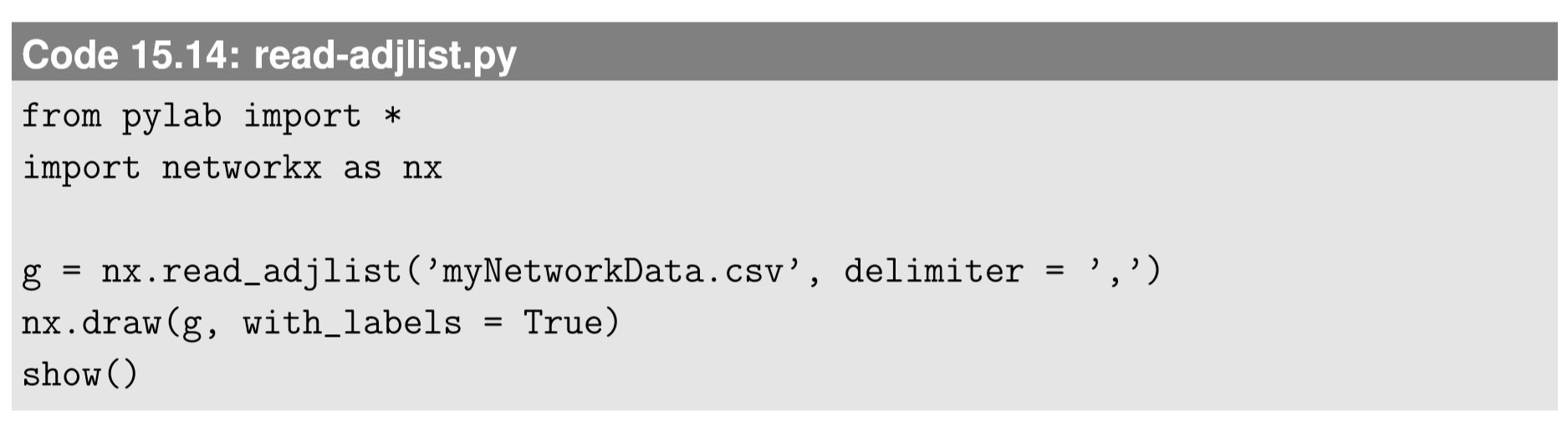
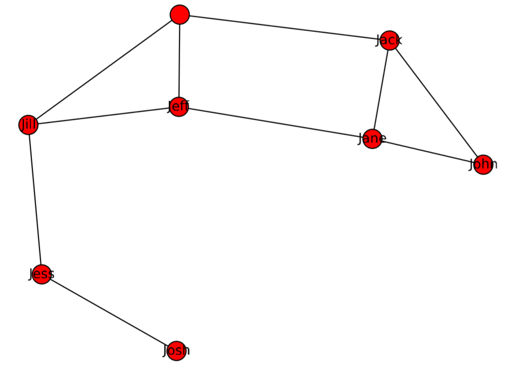
Looks good. No—wait—there is a problem here. For some reason, there is an extra node without a name (at the top of the network in Fig.15.5.3)! What happened? The reason becomes clear if you open the CSV file in a text editor, which reveals that the file actually looks like this:
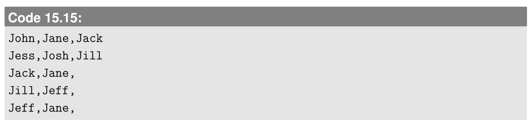
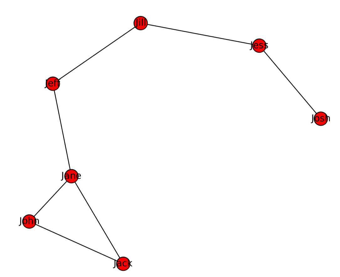
Note the commas at the end of the third, fourth, and fifth lines. Many spreadsheet applications tend to insert these extra commas in order to make the number of columns equal for all rows. This is why NetworkX thought there would be another node whose name was “” (blank). You can delete those unnecessary commas in the text editor and save the file. Or you could modify the visualization code to remove the nameless node before drawing the network. Either way, the updated result is shown in Fig. 15.5.4.
If you want to import the data as a directed graph, you can use the create_using option in the read_adjlist command, as follows:
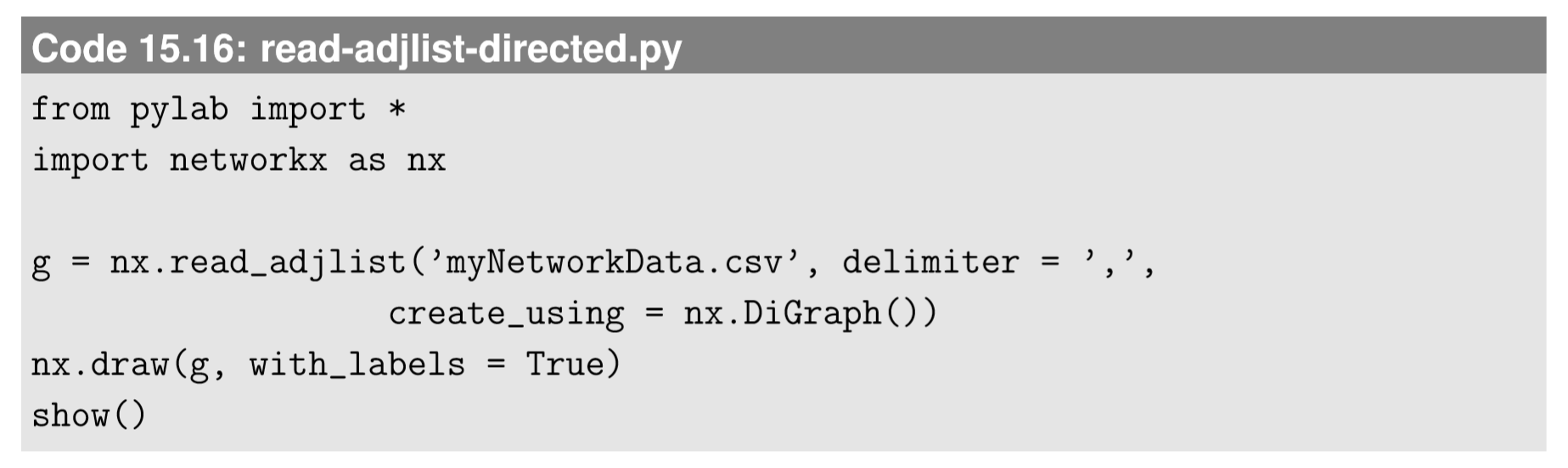
The result is shown in Fig.15.5.5, in which arrowheads are indicated by thick line segments.
Another simple function for data importing is read_edgelist. This function reads an edge list, i.e., a list of pairs of nodes, formatted as follows:


One useful feature of read_edgelist is that it can import not only edges but also their properties, such as:
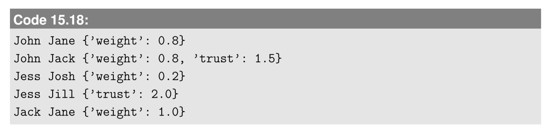
The third column of this data file is structured as a Python dictionary, which will be imported as the property of the edge.
Create a data file of the social network you created in Exercise 15.3.2 using a spreadsheet application, and then read the file and visualize it using NetworkX. You can use either the adjacency list format or the edge list format.
Import network data of your choice from Mark Newman’s Network Data website: http://www-personal.umich.edu/~mejn/netdata/. The data on this website are all in GML format, so you need to figure out how to import them into NetworkX. Then visualize the imported network.
Finally, NetworkX also has functions to write network data files from its graph objects, such as write_adjlist and write_edgelist. Their usage is very straightforward. Here is an example:
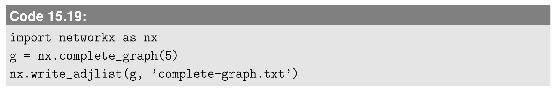
Then a new text file named ’complete-graph.txt’ will appear in the same folder, which looks like this:

Note that the adjacency list is optimized so that there is no redundant information included in this output. For example, node 4 is connected to 0, 1, 2, and 3, but this information is not included in the last line because it was already represented in the preceding lines.
Write the network data of Zachary’s Karate Club graph into a file in each of the following formats:
• Adjacency list
• Edge list
2For more details, see https://networkx.github.io/documenta...ence/readwrite. html.
3If you can’t read the data file or get the correct result, it may be because your NetworkX did not recognize operating system-specific newline characters in the file (this may occur particularly for Mac users). You can avoid this issue by saving the CSV file in a different mode (e.g., “MS-DOS” mode in Microsoft Excel).