
13.3: Range Versus Angle
- Page ID
- 119318

Now we’ll simulate the trajectory of the baseball with a range of launch angles. First, we’ll take the code we have and wrap it in a function that takes the launch angle as an input variable, runs the simulation, and returns the distance the ball travels (Listing 13.1).
Listing 13.1: A function that takes the launch angle of a baseball and returns the distance it travels
function res = baseball_range(theta)
    P = [0; 1];
    v = 50;
    [vx, vy] = pol2cart(theta, v);

    V = [vx; vy];     % initial velocity in m/s
    W = [P; V];       % initial condition

    tspan = [0 10];
    options = odeset('Events', @event_func);
    [T, M] = ode45(@rate_func, tspan, W, options);

    res = M(end, 1);
end
The launch angle, theta, is in radians. The magnitude of velocity, v, is always 50 m/s. We use pol2cart to convert the angle and magnitude (polar coordinates) to Cartesian components, vx and vy.
After running the simulation we extract the final \(x\)-position and return it as an output variable.
We can run this function for a range of angles like this:
    thetas = linspace(0, pi/2);
    for i = 1:length(thetas)
        ranges(i) = baseball_range(thetas(i));
    end
And then plot ranges as a function of thetas:
plot(thetas, ranges)Figure 13.2 shows the result. As expected, the ball does not travel far if it’s hit nearly horizontal or vertical. The peak is apparently near 0.7 rad.
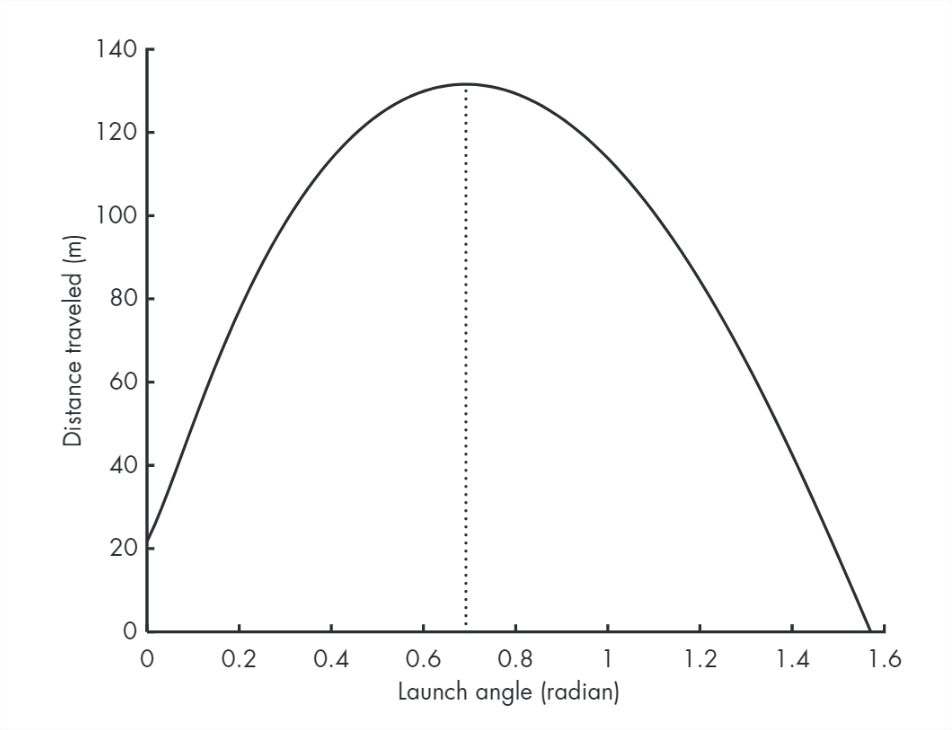 Figure 13.2: Simulated flight of a baseball plotted as a trajectory
Considering that our model is only approximate, this result might be good enough. But if we want to find the peak more precisely, we can use fminsearch.