17: Flow Past an Obstacle

We now consider a classic problem in computational fluid dynamics: the steady, two-dimensional flow past an obstacle. Here, we consider flows past a rectangle and a circle.

First, we consider flow past a rectangle. The simple Cartisian coordinate system is most suitable for this problem, and the boundaries of the internal rectangle can be aligned with the computational grid. Second, we consider flow past a circle. Here, the polar coordinate system is most suitable, and this introduces some additional analytical complications to the problem formulation. Nevertheless, we will see that the computation of flow past a circle may in fact be simpler than flow past a rectangle. Although flow past a rectangle contains two dimensionless parameters, flow past a circle contains only one. Furthermore, flow past a circle may be solved within a rectangular domain having no internal boundaries.

Flow past a rectangle

The free stream velocity is given by $\mathbf{u}=U \hat{\mathbf{x}}$ and the rectangular obstacle is assumed to have width $W$ and height $H$. Now, the stream function has units of velocity times length, and the vorticity has units of velocity divided by length. The steady, two-dimensional Poisson equations for the stream function and the vorticity, given by (16.14) and (16.18), may be nondimensionalized using the velocity $U$ and the length $W$. The resulting dimensionless equations can be written as

$$\begin{align} &-\nabla^{2} \psi=\omega, \\ &-\nabla^{2} \omega=\operatorname{Re}\left(\frac{\partial \psi}{\partial x} \frac{\partial \omega}{\partial y}-\frac{\partial \psi}{\partial y} \frac{\partial \omega}{\partial x}\right), \end{align} \nonumber$$

where the dimensionless parameter Re is called the Reynolds number. An additional dimensionless parameter arises from the aspect ratio of the rectangular obstacle, and is denoted by $a$. These two dimensionless parameters are defined by

$$\operatorname{Re}=\frac{U W}{V}, \quad a=\frac{W}{H} . \nonumber$$

A solution for the scalar stream function and scalar vorticity field will be sought for different values of the Reynolds number Re at a fixed aspect ratio $a$

Finite difference approximation

We construct a rectangular grid for a numerical solution. We will make use of square grid cells, and write

$$\begin{array}{ll} x_{i}=i h, & i=0,1, \ldots, N_{x} ; \\ y_{j}=j h, & j=0,1, \ldots, N_{y}, \end{array} \nonumber$$

where $N_{x}$ and $N_{y}$ are the number of grid cells spanning the $x$ - and $y$-directions, and $h$ is the side length of a grid cell.

To obtain an accurate solution, we require the boundaries of the obstacle to lie exactly on the boundaries of the grid cell. The width of the obstacle in our dimensionless formulation is unity, and we place the front of the obstacle at $x=m h$ and the back of the obstacle at $x=(m+I) h$, where we must have

$$h I=1 \text {. } \nonumber$$

With $I$ specified, the grid spacing is determined by $h=1 / I$.

We will only look for steady solutions for the flow field that are symmetric about the midline of the obstacle. Assuming symmetry, we need only solve for the flow field in the upper half of the domain. We place the center line of the obstacle at $y=0$ and the top of rectangle at $h J .$ The dimensionless half-height of the obstacle is given by $1 / 2 a$, so that

$$h J=\frac{1}{2 a} . \nonumber$$

Forcing the rectangle to lie on the grid lines constrains the choice of aspect ratio and the values of $I$ and $J$ such that

$$a=\frac{I}{2 J} \text {. } \nonumber$$

Reasonable values of $a$ to consider are $a=\ldots, 1 / 4,1 / 2,1,2,4, \ldots$, etc, and $I$ and $J$ can be adjusted accordingly.

The physics of the problem is specified through the two dimensionless parameters Re and $a$. The numerics of the problem is specified by the parameters $N_{x}, N_{y}, h$, and the placement of the rectangle in the computational domain. We look for convergence of the numerical solution as $h \rightarrow 0, N_{x}, N_{y} \rightarrow \infty$ and the rectangle is placed far from the boundaries of the computationally domain.

Discretizing the governing equations, we now write

$$\psi_{i, j}=\psi\left(x_{i}, y_{j}\right), \quad \omega_{i, j}=\omega\left(x_{i}, y_{j}\right) . \nonumber$$

To solve the coupled Poisson equations given by (17.1) and (17.2), we make use of the SOR method, previously described in §7.1. The notation we use here is for the Jacobi method, but faster convergence is likely to be achieved using red-back Gauss-Seidel. The Poisson equation for the stream function, given by (17.1), becomes

$$\psi_{i, j}^{n+1}=\left(1-r_{\psi}\right) \psi_{i, j}^{n}+\frac{r_{\psi}}{4}\left(\psi_{i+1, j}^{n}+\psi_{i-1, j}^{n}+\psi_{i, j+1}^{n}+\psi_{i, j-1}^{n}+h^{2} \omega_{i, j}^{n}\right) . \nonumber$$

The Poisson equation for the vorticity, given by $(17.2)$, requires use of the centered finite difference approximation for the derivatives that appear on the right-hand-side. For $x=x_{i}, y=y_{i}$, these approximations are given by

$$\begin{array}{ll} \frac{\partial \psi}{\partial x} \approx \frac{1}{2 h}\left(\psi_{i+1, j}-\psi_{i-1, j}\right), & \frac{\partial \psi}{\partial y} \approx \frac{1}{2 h}\left(\psi_{i, j+1}-\psi_{i, j-1}\right) \\ \frac{\partial \omega}{\partial x} \approx \frac{1}{2 h}\left(\omega_{i+1, j}-\omega_{i-1, j}\right), & \frac{\partial \omega}{\partial y} \approx \frac{1}{2 h}\left(\omega_{i, j+1}-\omega_{i, j-1}\right) . \end{array} \nonumber$$

We then write for (17.2),

$$\omega_{i, j}^{n+1}=\left(1-r_{\omega}\right) \omega_{i, j}^{n}+\frac{r_{\omega}}{4}\left(\omega_{i+1, j}^{n}+\omega_{i-1, j}^{n}+\omega_{i, j+1}^{n}+\omega_{i, j-1}^{n}+\frac{\operatorname{Re}}{4} f_{i, j}^{n}\right), \nonumber$$

where

$$f_{i j}^{n}=\left(\psi_{i+1, j}^{n}-\psi_{i-1, j}^{n}\right)\left(\omega_{i, j+1}^{n}-\omega_{i, j-1}^{n}\right)-\left(\psi_{i, j+1}^{n}-\psi_{i, j-1}^{n}\right)\left(\omega_{i+1, j}^{n}-\omega_{i-1, j}^{n}\right) \nonumber$$

Now, the right-hand-side of (17.11) contains a nonlinear term given by (17.12). This nonlinearity can result in the iterations becoming unstable.

The iterations can be stabilized as follows. First, the relaxation parameters, $r_{\psi}$ and $r_{\omega}$, should be less than or equal to unity, and unstable iterations can often be made stable by decreasing $r_{\omega}$. One needs to numerically experiment to obtain the best trade-off between computationally stability and speed. Second, to determine the solution with Reynolds number Re, the iteration should be initialized using the steady solution for a slightly smaller Reynolds number. Initial conditions for the first solution with Re slightly larger than zero should be chosen so that this first iteration is stable.

The path of convergence can be tracked during the iterations. We define

$$\begin{aligned} &\varepsilon_{\psi}^{n+1}=\max _{i, j}\left|\psi_{i, j}^{n+1}-\psi_{i, j}^{n}\right| \\ &\varepsilon_{\omega}^{n+1}=\max _{i, j}\left|\omega_{i, j}^{n+1}-\omega_{i, j}^{n}\right| . \end{aligned} \nonumber$$

The iterations are to be stopped when the values of $\varepsilon_{\psi}^{n+1}$ and $\varepsilon_{\omega}^{n+1}$ are less than some pre-defined error tolerance, say $10^{-8}$.

Boundary conditions

Boundary conditions on $\psi_{i, j}$ and $\omega_{i, j}$ must be prescribed at $i=0$ (inflow), $i=N_{x}$ (outflow), $j=0$ (midline), and $j=N_{y}$ (top of computational domain). Also, boundary conditions must be prescribed on the surface of the obstacle; that is, on the front surface: $i=m, 0 \leq j \leq I$; the back surface: $i=m+I, 0 \leq j \leq J$; and the top surface: $m \leq i \leq m+I, j=J .$ Inside of the obstacle, $m<i<m+I, 0<j<J$, no solution is sought.

For the inflow and top-of-domain boundary conditions, we may assume that the flow field satisfies dimensionless free-stream conditions; that is,

$$u=1, \quad v=0 . \nonumber$$

The vorticity may be taken to be zero, and the stream function satisfies

$$\frac{\partial \psi}{\partial y}=1, \quad \frac{\partial \psi}{\partial x}=0 \nonumber$$

Integrating the first of these equations, we obtain

$$\psi=y+f(x) ; \nonumber$$

and from the second equation we obtain $f(x)=c$, where $c$ is a constant. Without loss of generality, we may choose $c=0$. Therefore, for the inflow and top-of-domain boundary conditions, we have

$$\psi=y, \quad \omega=0 \nonumber$$

At the top of the domain, notice that $y=N_{y} h$ is a constant.

For the outflow boundary conditions, we have two possible choices. We could assume freestream conditions if we place the outflow boundary sufficiently far away from the obstacle. However, one would expect that the disturbance to the flow field downstream of the obstacle might be substantially greater than that upstream of the obstacle. Perhaps better outflow boundary conditions may be zero normal derivatives of the flow field; that is

$$\frac{\partial \psi}{\partial x}=0, \quad \frac{\partial \omega}{\partial x}=0 \nonumber$$

For the midline boundary conditions, we will assume a symmetric flow field so that the flow pattern will look the same when rotated about the $x$-axis. The symmetry conditions are therefore given by

$$u(x,-y)=u(x, y), \quad v(x,-y)=-v(x, y) . \nonumber$$

The vorticity exhibits the symmetry given by

$$\begin{aligned} \omega(x,-y) &=\frac{\partial v(x,-y)}{\partial x}-\frac{\partial u(x,-y)}{\partial(-y)} \\ &=-\frac{\partial v(x, y)}{\partial x}+\frac{\partial u(x, y)}{\partial(y)} \\ &=-\omega(x, y) \end{aligned} \nonumber$$

On the midline $(y=0)$, then, $\omega(x, 0)=0 .$ Also, $v(x, 0)=0 .$ With $v=-\partial \psi / \partial x$, we must have $\psi(x, 0)$ independent of $x$, or $\psi(x, 0)$ equal to a constant. Matching the midline boundary condition to our chosen inflow condition determines $\psi(x, 0)=0$.

Our boundary conditions are discretized using (17.4). The outflow condition of zero normal derivative could be approximated either to first- or second-order. Since it is an approximate boundary condition, first-order is probably sufficient and we use $\psi_{N_{x}, j}=\psi_{N_{x}-1, j}$ and $\omega_{N_{x}, j}=$ $\omega_{N_{x}-1, j} .$

Putting all these results together, the boundary conditions on the borders of the computational domain are given by

$$\begin{aligned} \psi_{i, 0} &=0, & \omega_{i, 0} &=0, & \text { midline; } \\ \psi_{0, j} &=j h, & \omega_{0, j} &=0, & \text { inflow; } \\ \psi_{N_{x}, j} &=\psi_{N_{x}-1, j,} & \omega_{N_{x}, j} &=\omega_{N_{x}-1, j \prime} & \text { outflow; } \\ \psi_{i, N_{y}} &=N_{y} h, & \omega_{i, N_{y}} &=0, & \text { top-of-domain. } \end{aligned} \nonumber$$

Boundary conditions on the obstacle can be derived from the no-penetration and no-slip conditions. From the no-penetration condition, $u=0$ on the sides and $v=0$ on the top. Therefore, on the sides, $\partial \psi / \partial y=0$, and since the side boundaries are parallel to the $y$-axis, $\psi$ must be constant. On the top, $\partial \psi / \partial x=0$, and since the top is parallel to the $x$-axis, $\psi$ must be constant. Matching the constant to the value of $\psi$ on the midline, we obtain $\psi=0$ along the boundary of the obstacle.

From the no-slip condition, $v=0$ on the sides and $u=0$ on the top. Therefore, $\partial \psi / \partial x=0$ on the sides and $\partial \psi / \partial y=0$ on the top. To interpret the no-slip boundary conditions in terms of boundary conditions on the vorticity, we make use of $(17.1)$; that is,

$$\omega=-\left(\frac{\partial^{2} \psi}{\partial x^{2}}+\frac{\partial^{2} \psi}{\partial y^{2}}\right) \nonumber$$

First consider the sides of the obstacle. Since $\psi$ is independent of $y$ we have $\partial^{2} \psi / \partial y^{2}=0$, and (17.19) becomes

$$\omega=-\frac{\partial^{2} \psi}{\partial x^{2}} \nonumber$$

We now Taylor series expand $\psi\left(x_{m}-h, y_{j}\right)$ and $\psi\left(x_{m}-2 h, y_{j}\right)$ about $\left(x_{m}, y_{j}\right)$, corresponding to the front face of the rectangular obstacle. We have to order $h^{3}$ :

$$\begin{aligned} &\psi_{m-1, j}=\psi_{m, j}-\left.h \frac{\partial \psi}{\partial x}\right|_{m, j}+\left.\frac{1}{2} h^{2} \frac{\partial^{2} \psi}{\partial x^{2}}\right|_{m, j}-\left.\frac{1}{6} h^{3} \frac{\partial^{3} \psi}{\partial x^{3}}\right|_{m, j}+\mathrm{O}\left(h^{4}\right), \\ &\psi_{m-2, j}=\psi_{m, j}-\left.2 h \frac{\partial \psi}{\partial x}\right|_{m, j}+\left.2 h^{2} \frac{\partial^{2} \psi}{\partial x^{2}}\right|_{m, j}-\left.\frac{4}{3} h^{3} \frac{\partial^{3} \psi}{\partial x^{3}}\right|_{m, j}+\mathrm{O}\left(h^{4}\right) . \end{aligned} \nonumber$$

The first terms in the two Taylor series expansions are zero because of the no-penetration condition, and the second terms are zero because of the no-slip condition. The third terms acan be rewritten using (17.20), and we obtain

$$\begin{aligned} &\psi_{m-1, j}=-\frac{1}{2} h^{2} \omega_{m, j}-\left.\frac{1}{6} h^{3} \frac{\partial^{3} \psi}{\partial x^{3}}\right|_{m, j}+\mathrm{O}\left(h^{4}\right) \\ &\psi_{m-2, j}=-2 h^{2} \omega_{m, j}-\left.\frac{4}{3} h^{3} \frac{\partial^{3} \psi}{\partial x^{3}}\right|_{m, j}+\mathrm{O}\left(h^{4}\right) \end{aligned} \nonumber$$

We multiply the first equation by $-8$ and add it to the second equation to eliminate the $h^{3}$ term. We obtain

$$-8 \psi_{m-1, j}+\psi_{m-2, j}=2 h^{2} \omega_{m, j}+\mathrm{O}\left(h^{4}\right) . \nonumber$$

Solving for the vorticity, we have a second-order accurate boundary condition given by

$$\omega_{m, j}=\frac{\psi_{m-2, j}-8 \psi_{m-1, j}}{2 h^{2}} \nonumber$$

Similar considerations applied to the back face of the rectangular obstacle yields

$$\omega_{m+1, j}=\frac{\psi_{m+I+2, j}-8 \psi_{m+I+1, j}}{2 h^{2}} \nonumber$$

On the top of the obstacle, $y=J h$ is fixed, and since $\psi$ is independent of $x$, we have $\partial^{2} \psi / \partial x^{2}=$ 0 . Therefore,

$$\omega=-\frac{\partial^{2} \psi}{\partial y^{2}} \nonumber$$

We now Taylor series expand $\psi\left(x_{i}, y_{J+1}\right)$ and $\psi\left(x_{i}, y_{J+2}\right)$ about $\left(x_{i}, y_{J}\right) .$ To order $h^{3}$,

$$\begin{aligned} &\psi_{i, J+1}=\psi_{i, J}+\left.h \frac{\partial \psi}{\partial y}\right|_{i, J}+\left.\frac{1}{2} h^{2} \frac{\partial^{2} \psi}{\partial y^{2}}\right|_{i, J}+\left.\frac{1}{6} h^{3} \frac{\partial^{3} \psi}{\partial y^{3}}\right|_{i, J}+\mathrm{O}\left(h^{4}\right), \\ &\psi_{i, J+2}=\psi_{i, J}+\left.2 h \frac{\partial \psi}{\partial y}\right|_{i, J}+\left.2 h^{2} \frac{\partial^{2} \psi}{\partial y^{2}}\right|_{i, J}+\left.\frac{4}{3} h^{3} \frac{\partial^{3} \psi}{\partial y^{3}}\right|_{i, J}+\mathrm{O}\left(h^{4}\right) . \end{aligned} \nonumber$$

Again, the first and second terms in the Taylor series expansion are zero, and making use of (17.24), we obtain

$$\begin{aligned} &\psi_{i, J+1}=-\frac{1}{2} h^{2} \omega_{i, J}+\left.\frac{1}{6} h^{3} \frac{\partial^{3} \psi}{\partial y^{3}}\right|_{i, J}+\mathrm{O}\left(h^{4}\right), \\ &\psi_{i, J+2}=-2 h^{2} \omega_{i, J}+\left.\frac{4}{3} h^{3} \frac{\partial^{3} \psi}{\partial y^{3}}\right|_{i, J}+\mathrm{O}\left(h^{4}\right) . \end{aligned} \nonumber$$

Again, we multiply the first equation by $-8$ and add it to the second equation to obtain

$$-8 \psi_{i, J+1}+\psi_{i, J+2}=2 h^{2} \omega_{i, J}+\mathrm{O}\left(h^{4}\right) \nonumber$$

Solving for the vorticity on the top surface, we have to second-order accuracy

$$\omega_{i, J}=\frac{\psi_{i, J+2}-8 \psi_{i, J+1}}{2 h^{2}} \nonumber$$

We summarize the boundary conditions on the obstacle:

$$\begin{array}{cc} \text { front face: } \psi_{m, j}=0, & \omega_{m, j}=\frac{\psi_{m-2, j}-8 \psi_{m-1, j}}{2 h^{2}}, \quad 0 \leq j \leq J ; \\ \text { back face: } \psi_{m+I, j}=0, & \omega_{m+I, j}=\frac{\psi_{m+I+2, j}-8 \psi_{m+I+1, j}}{2 h^{2}}, \quad 0 \leq j \leq J ; \\ \text { top face: } \psi_{i, J}=0, & \omega_{i, J}=\frac{\psi_{i, J+2}-8 \psi_{i, J+1}}{2 h^{2}}, \quad m \leq i \leq m+I . \end{array} \nonumber$$

Flow past a circle

We now consider flow past a circular obstacle of radius $R$, with free-stream velocity $\mathbf{u}=U \hat{\mathbf{x}}$ Here, we nondimensionalize the governing equations using $U$ and $R$. We will define the Reynolds number-the only dimensionless parameter of this problem-by

$$\operatorname{Re}=\frac{2 U R}{v} . \nonumber$$

The extra factor of 2 bases the definition of the Reynolds number on the diameter of the circle rather than the radius, which allows a better comparison to computations of flow past a square $(a=1)$, where the Reynolds number was based on the side length

The dimensionless governing equations in vector form, can be written as

$$\begin{align} \nonumber \nabla^{2} \psi &=-\omega \\ \nabla^{2} \omega &=\frac{\operatorname{Re}}{2} \mathbf{u} \cdot \nabla \omega \end{align} \nonumber$$

where the extra factor of one-half arises from nondimensionalizing the equation using the radius of the obstacle $R$, but defining the Reynolds number in terms of the diameter $2 R$.

Log-polar coordinates

Although the free-stream velocity is best expressed in Cartesian coordinates, the boundaries of the circular obstacle are more simply expressed in polar coordinates, with origin at the center of the circle. Polar coordinates are defined in the usual way by

$$x=r \cos \theta, \quad y=r \sin \theta, \nonumber$$

with the cartesian unit vectors given in terms of the polar unit vectors by

$$\hat{\mathbf{x}}=\cos \theta \hat{\mathbf{r}}-\sin \theta \hat{\boldsymbol{\theta}}, \quad \hat{\boldsymbol{y}}=\sin \theta \hat{\mathbf{r}}+\cos \theta \hat{\boldsymbol{\theta}} \nonumber$$

The polar unit vectors are functions of position, and their derivatives are given by

$$\frac{\partial \hat{\mathbf{r}}}{\partial r}=0, \quad \frac{\partial \hat{\mathbf{r}}}{\partial \theta}=\hat{\boldsymbol{\theta}}, \quad \frac{\partial \hat{\boldsymbol{\theta}}}{\partial r}=0, \quad \frac{\partial \hat{\boldsymbol{\theta}}}{\partial \theta}=-\hat{\mathbf{r}} \nonumber$$

The del differential operator in polar coordinates is given by

$$\boldsymbol{\nabla}=\hat{\mathbf{r}} \frac{\partial}{\partial r}+\hat{\theta} \frac{1}{r} \frac{\partial}{\partial \theta} \nonumber$$

and the two-dimensional Laplacian is given by

$$\nabla^{2}=\frac{1}{r^{2}}\left(\left(r \frac{\partial}{\partial r}\right)\left(r \frac{\partial}{\partial r}\right)+\frac{\partial^{2}}{\partial \theta^{2}}\right) \nonumber$$

The velocity field is written in polar coordinates as

$$\mathbf{u}=u_{r} \hat{\mathbf{r}}+u_{\theta} \hat{\theta} \nonumber$$

The free-stream velocity in polar coordinates is found to be

$$\begin{align} \nonumber \mathbf{u} &=U \hat{\mathbf{x}} \\ &=U(\cos \theta \hat{\mathbf{r}}-\sin \theta \hat{\boldsymbol{\theta}}), \end{align} \nonumber$$

from which can be read off the components in polar coordinates. The continuity equation $\boldsymbol{\nabla} \cdot \mathbf{u}=$ 0 in polar coordinates is given by

$$\frac{1}{r} \frac{\partial}{\partial r}\left(r u_{r}\right)+\frac{1}{r} \frac{\partial u_{\theta}}{\partial \theta}=0 \nonumber$$

so that the stream function can be defined by

$$r u_{r}=\frac{\partial \psi}{\partial \theta}, \quad u_{\theta}=-\frac{\partial \psi}{\partial r} . \nonumber$$

The vorticity, here in cylindrical coordinates, is given by

$$\begin{aligned} \omega &=\nabla \times \mathbf{u} \\ &=\hat{\mathbf{z}}\left(\frac{1}{r} \frac{\partial}{\partial r}\left(r u_{\theta}\right)-\frac{1}{r} \frac{\partial u_{r}}{\partial \theta}\right), \end{aligned} \nonumber$$

so that the z-component of the vorticity for a two-dimensional flow is given by

$$\omega=\frac{1}{r} \frac{\partial}{\partial r}\left(r u_{\theta}\right)-\frac{1}{r} \frac{\partial u_{r}}{\partial \theta} . \nonumber$$

Furthermore,

$$\begin{align} \nonumber \mathbf{u} \cdot \nabla &=\left(u_{r} \hat{\mathbf{r}}+u_{\theta} \hat{\boldsymbol{\theta}}\right) \cdot\left(\hat{\mathbf{r}} \frac{\partial}{\partial r}+\hat{\theta} \frac{1}{r} \frac{\partial}{\partial \theta}\right) \\ \nonumber &=u_{r} \frac{\partial}{\partial r}+\frac{u_{\theta}}{r} \frac{\partial}{\partial \theta} \\ &=\frac{1}{r} \frac{\partial \psi}{\partial \theta} \frac{\partial}{\partial r}-\frac{1}{r} \frac{\partial \psi}{\partial r} \frac{\partial}{\partial \theta} \end{align} \nonumber$$

The governing equations given by (17.29), then, with the Laplacian given by (17.34), and the convection term given by (17.40), are

$$\begin{align} \nabla^{2} \psi &=-\omega \\ \nabla^{2} \omega &=\frac{\operatorname{Re}}{2}\left(\frac{1}{r} \frac{\partial \psi}{\partial \theta} \frac{\partial \omega}{\partial r}-\frac{1}{r} \frac{\partial \psi}{\partial r} \frac{\partial \omega}{\partial \theta}\right) \end{align} \nonumber$$

The recurring factor $r \partial / \partial r$ in the polar coordinate Laplacian, (17.34), is awkward to discretize and we look for a change of variables $r=r(\xi)$, where

$$r \frac{\partial}{\partial r}=\frac{\partial}{\partial \xi} . \nonumber$$

Now,

$$\frac{\partial}{\partial \xi}=\frac{d r}{d \xi} \frac{\partial}{\partial r} \nonumber$$

so that we require

$$\frac{d r}{d \xi}=r \text {. } \nonumber$$

This simple differential equation can be solved if we take as our boundary condition $\xi=0$ when $r=1$, corresponding to points lying on the boundary of the circular obstacle. The solution of $(17.45)$ is therefore given by

$$r=e^{\zeta} \nonumber$$

The Laplacian in the so-called log polar coordinates then becomes

$$\begin{aligned} \nabla^{2} &=\frac{1}{r^{2}}\left(\left(r \frac{\partial}{\partial r}\right)\left(r \frac{\partial}{\partial r}\right)+\frac{\partial^{2}}{\partial \theta^{2}}\right) \\ &=e^{-2 \zeta}\left(\frac{\partial^{2}}{\partial \xi^{2}}+\frac{\partial^{2}}{\partial \theta^{2}}\right) . \end{aligned} \nonumber$$

Also, transforming the right-hand-side of $(17.42)$, we have

$$\begin{aligned} \frac{1}{r} \frac{\partial \psi}{\partial \theta} \frac{\partial \omega}{\partial r}-\frac{1}{r} \frac{\partial \psi}{\partial r} \frac{\partial \omega}{\partial \theta} &=\frac{1}{r^{2}}\left(r \frac{\partial \omega}{\partial r} \frac{\partial \psi}{\partial \theta}-r \frac{\partial \psi}{\partial r} \frac{\partial \omega}{\partial \theta}\right) \\ &=e^{-2 \xi}\left(\frac{\partial \psi}{\partial \theta} \frac{\partial \omega}{\partial \zeta}-\frac{\partial \psi}{\partial \xi} \frac{\partial \omega}{\partial \theta}\right) . \end{aligned} \nonumber$$

The governing equations for $\psi=\psi(\xi, \theta)$ and $\omega=\omega(\xi, \theta)$ in log-polar coordinates can therefore be written as

$$\begin{align} -&\left(\frac{\partial^{2}}{\partial \xi^{2}}+\frac{\partial^{2}}{\partial \theta^{2}}\right) \psi=e^{2 \xi} \omega \\ -&\left(\frac{\partial^{2}}{\partial \xi^{2}}+\frac{\partial^{2}}{\partial \theta^{2}}\right) \omega=\frac{\operatorname{Re}}{2}\left(\frac{\partial \psi}{\partial \xi} \frac{\partial \omega}{\partial \theta}-\frac{\partial \psi}{\partial \theta} \frac{\partial \omega}{\partial \xi}\right) . \end{align} \nonumber$$

Finite difference approximation

A finite difference approximation to the governing equations proceeds on a grid in $(\xi, \theta)$ space. The grid is defined for $0 \leq \xi \leq \zeta_{m}$ and $0 \leq \theta \leq \pi$, so that the computational domain forms a rectangle without holes. The sides of the rectangle correspond to the boundary of the circular obstacle $(\xi=0)$, the free stream $\left(\xi=\xi_{m}\right)$, the midline behind the obstacle $(\theta=0)$, and the midline in front of the obstacle $(\theta=\pi)$.

We discretize the equations using square grid cells, and write

$$\begin{array}{ll} \xi_{i}=i h, & i=0,1, \ldots, n \\ \theta_{j}=j h, & j=0,1, \ldots, m \end{array} \nonumber$$

where $n$ and $m$ are the number of grid cells spanning the $\xi$ - and $\theta$-directions, and $h$ is the side length of a grid cell. Because $0 \leq \theta \leq \pi$, the grid spacing must satisfy

$$h=\frac{\pi}{m} \nonumber$$

and the maximum value of $\xi$ is given by

$$\xi_{\max }=\frac{n \pi}{m} \nonumber$$

The radius of the computational domain is therefore given by $e^{\xi \max }$, which is to be compared to the obstacle radius of unity. The choice $n=m$ would yield $e^{\zeta_{\max }} \approx 23$, and the choice $n=2 m$ would yield $e^{\zeta_{\max }} \approx 535$. To perform an accurate computation, it is likely that both the value of $m$ (and $n$ ) and the value of $\xi_{\max }$ will need to increase with Reynolds number.

Again we make use of the SOR method, using the notation for the Jacobi method, although faster convergence is likely to be achieved using red-black Gauss-Seidel. The finite difference approximation to $(17.47 and 14.48)$ thus becomes

$$\psi_{i, j}^{n+1}=\left(1-r_{\psi}\right) \psi_{i, j}^{n}+\frac{r_{\psi}}{4}\left(\psi_{i+1, j}^{n}+\psi_{i-1, j}^{n}+\psi_{i, j+1}^{n}+\psi_{i, j-1}^{n}+h^{2} e^{2 \xi_{i}} \omega_{i, j}^{n}\right), \nonumber$$

and

$$\omega_{i, j}^{n+1}=\left(1-r_{\omega}\right) \omega_{i, j}^{n}+\frac{r_{\omega}}{4}\left(\omega_{i+1, j}^{n}+\omega_{i-1, j}^{n}+\omega_{i, j+1}^{n}+\omega_{i, j-1}^{n}+\frac{\operatorname{Re}}{8} f_{i, j}^{n}\right), \nonumber$$

Where

$$f_{i j}^{n}=\left(\psi_{i+1, j}^{n}-\psi_{i-1, j}^{n}\right)\left(\omega_{i, j+1}^{n}-\omega_{i, j-1}^{n}\right)-\left(\psi_{i, j+1}^{n}-\psi_{i, j-1}^{n}\right)\left(\omega_{i+1, j}^{n}-\omega_{i-1, j}^{n}\right) \nonumber$$

Boundary conditions

Boundary conditions must be prescribed on the sides of the rectangular computational domain The boundary conditions on the two sides corresponding to the midline of the physical domain, $\theta=0$ and $\theta=\pi$, satisfy $\psi=0$ and $\omega=0$. The boundary condition on the side corresponding to the circular obstacle, $\xi=0$, is again determined from the no-penentration and no-slip conditions, and are given by $\psi=0$ and $\partial \psi / \partial \xi^{\tau}=0 .$ And the free-stream boundary condition may be applied at $\xi=\xi_{\max }$.

We first consider the free-stream boundary condition. The dimensionless free-stream velocity field in polar coordinates can be found from (17.36),

$$\mathbf{u}=\cos \theta \hat{\mathbf{r}}-\sin \theta \hat{\boldsymbol{\theta}} \nonumber$$

The stream function, therefore, satisfies the free-stream conditions

$$\frac{\partial \psi}{\partial \theta}=r \cos \theta, \quad \frac{\partial \psi}{\partial r}=\sin \theta, \nonumber$$

and by inspection, the solution that also satisfies $\psi=0$ when $\theta=0, \pi$ is given by

$$\psi(r, \theta)=r \sin \theta . \nonumber$$

In log-polar coordinates, we therefore have the free-stream boundary condition

$$\psi\left(\xi_{\max }, \theta\right)=e^{\xi_{\max }} \sin \theta \nonumber$$

One has two options for the vorticity in the free stream. One could take the vorticity in the free stream to be zero, so that

$$\omega\left(\xi_{\max }, \theta\right)=0 \nonumber$$

A second, more gentle option is to take the derivative of the vorticity to be zero, so that

$$\frac{\partial \omega}{\partial \xi}\left(\xi_{\max }, \theta\right)=0 \nonumber$$

This second option seems to have somewhat better stability properties for the flow field far downstream of the obstacle. Ideally, the computed values of interest should be independent of which of these boundary conditions is chosen, and finding flow-field solutions using both of these boundary conditions provides a good measure of accuracy. The remaining missing boundary condition is for the vorticity on the obstacle. Again, we need to convert the two boundary conditions on the stream function, $\psi=0$ and $\partial \psi / \partial \xi=0$ to a boundary condition on $\psi$ and $\omega$. From (17.47 and 17.48), we have

$$\omega=-e^{-2 \tilde{}}\left(\frac{\partial^{2} \psi}{\partial \tilde{\xi}^{2}}+\frac{\partial^{2} \psi}{\partial \theta^{2}}\right) \nonumber$$

and since on the circle $\psi=0$, independent of $\theta$, and $\xi=0$, we have

$$\omega=-\frac{\partial^{2} \psi}{\partial \xi^{2}} \nonumber$$

A Taylor series expansion one and two grid points away from the circular obstacle yields

$$\begin{aligned} &\psi_{1, j}=\psi_{0, j}+\left.h \frac{\partial \psi}{\partial \xi}\right|_{(0, j)}+\left.\frac{1}{2} h^{2} \frac{\partial^{2} \psi}{\partial \xi^{2}}\right|_{(0, j)}+\left.\frac{1}{6} h^{3} \frac{\partial^{3} \psi}{\partial \xi^{3}}\right|_{(0, j)}+\mathrm{O}\left(h^{4}\right), \\ &\psi_{2, j}=\psi_{0, j}+\left.2 h \frac{\partial \psi}{\partial \xi}\right|_{(0, j)}+\left.2 h^{2} \frac{\partial^{2} \psi}{\partial \xi^{2}}\right|_{(0, j)}+\left.\frac{4}{3} h^{3} \frac{\partial^{3} \psi}{\partial \xi^{3}}\right|_{(0, j)}+\mathrm{O}\left(h^{4}\right) . \end{aligned} \nonumber$$

Now, both $\psi=0$ and $\partial \psi / \partial \xi=0$ at the grid point $(0, j) .$ Using the equation for the vorticity on the circle, $(17.62)$, results in

$$\begin{aligned} &\psi_{1, j}=-\frac{1}{2} h^{2} \omega_{0, j}+\left.\frac{1}{6} h^{3} \frac{\partial^{3} \psi}{\partial \zeta^{3}}\right|_{(0, j)}+\mathrm{O}\left(h^{4}\right), \\ &\psi_{2, j}=-2 h^{2} \omega_{0, j}+\left.\frac{4}{3} h^{3} \frac{\partial^{3} \psi}{\partial \xi^{3}}\right|_{(0, j)}+\mathrm{O}\left(h^{4}\right) . \end{aligned} \nonumber$$

We multiply the first equation by $-8$ and add it to the second equation to eliminate the $h^{3}$ term. We obtain

$$-8 \psi_{1, j}+\psi_{2, j}=2 h^{2} \omega_{0, j}+\mathrm{O}\left(h^{4}\right) \nonumber$$

Solving for the vorticity, we obtain our boundary condition accurate to second order:

$$\omega_{0, j}=\frac{\psi_{2, j}-8 \psi_{1, j}}{2 h^{2}} \nonumber$$

The boundary conditions are summarized below:

$$\begin{align} \nonumber \xi=0,0 \leq \theta \leq \pi: & \psi_{0, j}=0, \quad \omega_{0, j}=\frac{\psi_{2, j}-8 \psi_{1, j}}{2 h^{2}} ; \\ \xi=\xi_{\max }, 0 \leq \theta \leq \pi: & \psi_{n, j}=e^{\xi_{\max }} \sin j h, \quad \omega_{n, j}=0 \text { or } \omega_{n, j}=\omega_{n-1, j} ; \\ \nonumber 0 \leq \xi \leq \xi_{\max }, \theta=0: & \psi_{i, 0}=0, \quad \omega_{i, 0}=0 ; \\ \nonumber 0 \leq \xi \leq \xi_{\max }, \theta=\pi: & \psi_{i, m}=0, \quad \omega_{i, m}=0 . \end{align} \nonumber$$

Solution using Newton’s method

We consider here a much more efficient method to find the steady fluid flow solution. Unfortunately, this method is also more difficult to program. Recall from $\S 7.2$ that Newton’s method can be used to solve a system of nonlinear equations. Newton’s method as a root-finding routine has the strong advantage of being very fast when it converges, but the disadvantage of not always converging. Here, the problem of convergence can be overcome by solving for larger Re using as an initial guess the solution for slightly smaller Re, with slightly to be defined by trial and error. Recall that Newton’s method can solve a system of nonlinear equations of the form

$$F(\psi, \omega)=0, \quad G(\psi, \omega)=0 \nonumber$$

Newton’s method is implemented by writing

$$\psi^{(k+1)}=\psi^{(k)}+\Delta \psi, \quad \omega^{(k+1)}=\omega^{(k)}+\Delta \omega, \nonumber$$

and the iteration scheme is derived by linearizing $(17.66)$ in $\Delta \psi$ and $\Delta \omega$ to obtain

$$\mathrm{J}\left(\begin{array}{c} \Delta \psi \\ \Delta \omega \end{array}\right)=-\left(\begin{array}{l} F \\ G \end{array}\right) \nonumber$$

where $J$ is the Jacobian matrix of the functions $F$ and $G$. All functions are evaluated at $\psi^{(k)}$ and $\omega^{(k)}$.

Here, we should view $\psi$ and $\omega$ as a large number of unknowns and $F$ and $G$ a correspondingly large number of equations, where the total number of equations must necessarily equal the total number of unknowns.

If we rewrite our governing equations into the form given by (17.66), we have

$$\begin{align} \nonumber &-\left(\frac{\partial^{2}}{\partial \xi^{2}}+\frac{\partial^{2}}{\partial \theta^{2}}\right) \psi-e^{2 \xi} \omega=0 \\ &-\left(\frac{\partial^{2}}{\partial \tilde{\xi}^{2}}+\frac{\partial^{2}}{\partial \theta^{2}}\right) \omega-\frac{\operatorname{Re}}{2}\left(\frac{\partial \psi}{\partial \xi} \frac{\partial \omega}{\partial \theta}-\frac{\partial \psi}{\partial \theta} \frac{\partial \omega}{\partial \xi}\right)=0 \end{align} \nonumber$$

With $n$ and $m$ grid cells in the $\xi$ - and $\theta$-directions, the partial differential equations of (17.69) represent $2(n-1)(m-1)$ coupled nonlinear equations for $\psi_{i, j}$ and $\omega_{i, j}$ on the internal grid points. We will also include the boundary values in the solution vector that will add an additional two unknowns and two equations for each boundary point, bringing the total number of equations (and unknowns) to $2(n+1)(m+1)$.

The form of the Jacobian matrix may be determined by linearizing (17.69) in $\Delta \psi$ and $\Delta \omega$. Using $(17.67)$, we have

$$-\left(\frac{\partial^{2}}{\partial \xi^{2}}+\frac{\partial^{2}}{\partial \theta^{2}}\right)\left(\psi^{(k)}+\Delta \psi\right)-e^{2 \xi}\left(\omega^{(k)}+\Delta \omega\right)=0 \nonumber$$

and

$$\begin{aligned} -\left(\frac{\partial^{2}}{\partial \xi^{2}}+\frac{\partial^{2}}{\partial \theta^{2}}\right)\left(\omega^{(k)}+\Delta \omega\right) & \\ &-\frac{\operatorname{Re}}{2}\left(\frac{\partial\left(\psi^{(k)}+\Delta \psi\right)}{\partial \xi} \frac{\partial\left(\omega^{(k)}+\Delta \omega\right)}{\partial \theta}-\frac{\partial\left(\psi^{(k)}+\Delta \psi\right)}{\partial \theta} \frac{\partial\left(\omega^{(k)}+\Delta \omega\right)}{\partial \xi}\right)=0 . \end{aligned} \nonumber$$

Liinearization in $\Delta \psi$ and $\Delta \omega$ then results in

$$-\left(\frac{\partial^{2}}{\partial \xi^{2}}+\frac{\partial^{2}}{\partial \theta^{2}}\right) \Delta \psi-e^{2 \xi} \Delta \omega=-\left[-\left(\frac{\partial^{2}}{\partial \xi^{2}}+\frac{\partial^{2}}{\partial \theta^{2}}\right) \psi^{(k)}-e^{2 \xi} \omega^{(k)}\right] \nonumber$$

and

$$\begin{align} -\left(\frac{\partial^{2}}{\partial \xi^{2}}+\frac{\partial^{2}}{\partial \theta^{2}}\right) \Delta \omega &-\frac{\operatorname{Re}}{2}\left(\frac{\partial \omega^{(k)}}{\partial \theta} \frac{\partial \Delta \psi}{\partial \zeta}-\frac{\partial \omega^{(k)}}{\partial \xi} \frac{\partial \Delta \psi}{\partial \theta}+\frac{\partial \psi^{(k)}}{\partial \xi} \frac{\partial \Delta \omega}{\partial \theta}-\frac{\partial \psi^{(k)}}{\partial \theta} \frac{\partial \Delta \omega}{\partial \xi}\right) \nonumber \\ &=-\left[-\left(\frac{\partial^{2}}{\partial \xi ^{2}}+\frac{\partial^{2}}{\partial \theta^{2}}\right) \omega^{(k)}-\frac{\operatorname{Re}}{2}\left(\frac{\partial \psi^{(k)}}{\partial \xi} \frac{\partial \omega^{(k)}}{\partial \theta}-\frac{\partial \psi^{(k)}}{\partial \theta} \frac{\partial \omega^{(k)}}{\partial \xi}\right)\right] \end{align} \nonumber$$

where the first equation was already linear in the $\Delta$ variables, but the second equation was originally quadratic, and the quadratic terms have now been dropped. The equations given by (17.71) and (17.72) can be observed to be in the form of the Newton’s iteration equations given by (17.68).

Numerically, both $\Delta \psi$ and $\Delta \omega$ will be vectors formed by a natural ordering of the grid points, as detailed in $\$ 6.2$. These two vectors will then be stacked into a single vector as shown in (17.68). To write the Jacobian matrix, we employ the shorthand notation $\partial_{\tau}^{2}=\partial^{2} / \partial \xi^{2}, \psi_{\xi}=\partial \psi / \partial \xi$, and so on. The Jacobian matrix can then be written symbolically as

$$\mathrm{J}=\left(\begin{array}{cc} -\left(\partial_{\xi}^{2}+\partial_{\theta}^{2}\right) & -e^{2 \xi} \mathrm{I} \\ 0 & -\left(\partial_{\xi}^{2}+\partial_{\theta}^{2}\right) \end{array}\right) \quad-\frac{\operatorname{Re}}{2}\left(\begin{array}{cc} 0 & 0 \\ \omega_{\theta} \partial_{\xi}-\omega_{\xi} \partial_{\theta} & \psi_{\xi} \partial_{\theta}-\psi_{\theta} \partial_{\xi} \end{array}\right) \nonumber$$

where I is the identity matrix and the derivatives of $\psi$ and $\omega$ in the second matrix are all evaluated at the $k$ th iteration.

The Jacobian matrix as written is valid for the grid points interior to the boundary, where each row of J corresponds to an equation for either $\psi$ or $\omega$ at a specific interior grid point. The Laplacian-like operator is represented by a Laplacian matrix, and the derivative operators are represented by derivative matrices. The terms $e^{2 \xi}, \partial \omega / \partial \theta$, and the other derivative terms are to be evaluated at the grid point corresponding to the row in which they are found.

To incorporate boundary conditions, we extend the vectors $\Delta \psi$ and $\Delta \omega$ to also include the points on the boundary as they occur in the natural ordering of the grid points. To the Jacobian matrix and the right-hand-side of (17.68) are then added the appropriate equations for the boundary conditions in the rows corresponding to the boundary points. By explicitly including the boundary points in the solution vector, the second-order accurate Laplacian matrix and derivative matrices present in J can handle the grid points lying directly next to the boundaries without special treatment.

The relevant boundary conditions to be implemented are the boundary conditions on $\Delta \psi$ and $\Delta \omega$. The boundary conditions on the fields $\psi$ and $\omega$ themselves have already been given by (17.65). The grid points with fixed boundary conditions on $\psi$ and $\omega$ that do not change with iterations will have a one on the diagonal in the Jacobian matrix corresponding to that grid point, and a zero on the right-hand-side. In other words, $\psi$ and $\omega$ will not change on iteration of Newton’s method, and their initial values need to be chosen to satisfy the appropriate boundary conditions.

The two boundary conditions which change on iteration, namely

$$\omega_{0, j}=\frac{\psi_{2, j}-8 \psi_{1, j}}{2 h^{2}}, \quad \omega_{n, j}=\omega_{n-1, j} \nonumber$$

must be implemented in the Newton’s method iteration as

$$\Delta \omega_{0, j}=\frac{\Delta \psi_{2, j}-8 \Delta \psi_{1, j}}{2 h^{2}}, \quad \Delta \omega_{n, j}=\Delta \omega_{n-1, j} \nonumber$$

and these equations occur in the rows corresponding to the grid points $(0, j)$ and $(n, j)$, with $j=0$ to $m$. Again, the initial conditions for the iteration must satisfy the correct boundary conditions.

The MATLAB implementation of (17.68) using (17.73), requires both the construction of the $(n+1)(m+1) \times(n+1)(m+1)$ matrix that includes both the Jacobian matrix and the boundary conditions, and the construction of the corresponding right-hand-side of the equation. For the Laplacian matrix, one can make use of the function sp_laplace_new.m; and one also needs to construct the derivative matrices $\partial_{\xi}$ and $\partial_{\theta}$. Both of these matrices are banded, with a band of positive ones above the main diagonal and a band of negative ones below the main diagonal. For $\partial_{\xi}$, the bands are directly above and below the diagonal. For $\partial_{\theta}$, the bands are a distance $n+1$ away from the diagonal, corresponding to $n+1$ grid points in each row. Both the Laplacian and derivative matrices are to be constructed for $(n+1) \times(m+1)$ grid points and placed into a $2 \times 2$ matrix using the MATLAB function kron.m, which generates a block matrix by implementing the so-called Kronecker product. Rows corresponding to the boundary points are then to be replaced by the equations for the boundary conditions.

The MATLAB code needs to be written efficiently, using sparse matrices. A profiling of this code should show that most of the computational time is spent solving (17.68) (with boundary conditions added) for $\Delta \psi$ and $\Delta \omega$ using the MATLAB backslash operator. With $4 \mathrm{~GB}$ RAM and a notebook computer bought circa 2013 , and with the resolution $512 \times 256$ and using the $R e=150$ result as the initial field, I can solve for $R e=200$ in seven iterations to an accuracy of $10^{-12}$. The total run time was about $48 \mathrm{sec}$ with about $42 \mathrm{sec}$ spent on the single line containing $J \backslash \mathrm{b}$.

Visualization of the flow fields

Obtaining correct contour plots of the stream function and vorticity can be a challenge and in this section I will provide some guidance. The basic MATLAB functions required are meshgrid.m, pol2cart.m, contour.m, and clabel.m. More fancy functions such as contourf.m and imagesc may also be used, though I will not discuss these here.

Suppose the values of the stream function are known on a grid in two dimensional Cartesian coordinates. A contour plot draws curves following specified (or default) constant values of the stream function in the $x-y$ plane. Viewing the curves on which the stream function is constant gives a clear visualization of the fluid flow.

To make the best use of the function contour.m, one specifies the $x-y$ grid on which the values of the stream function are known. The stream function variable psi, say, is given as an $n$-by- $m$ matrix. We will examine a simple example to understand how to organize the data.

Let us assume that the stream function is known at all the values of $x$ and $y$ on the twodimensional grid specified by $x=[0,1,2]$ and $y=[0,1]$. To properly label the axis of the contour plot, we use the function meshgrid, and write $[X, Y]=\operatorname{meshgrid}(X, Y)$. The values assigned to $X$ and $Y$ are the following 2 -by-3 matrices:

$$X=\left[\begin{array}{lll} 0 & 1 & 2 \\ 0 & 1 & 2 \end{array}\right], \quad Y=\left[\begin{array}{lll} 0 & 0 & 0 \\ 1 & 1 & 1 \end{array}\right] \nonumber$$

The variable psi must have the same dimensions as the variables $X$ and $Y$. Suppose psi is given by

$$\text { psi }=\left[\begin{array}{lll} a & b & c \\ d & e & f \end{array}\right] \nonumber$$

Then the data must be organized so that psi $=a$ at $(x, y)=(0,0)$, psi $=b$ at $(x, y)=(1,0)$, psi $=d$ at $(x, y)=(0,1)$, etc. Notice that the values of psi across a row $(\mathrm{psi}(i, j), j=1: 3)$ correspond to different $x$ locations, and the values of psi down a column $((p s i(i, j), i=1: 2))$ correspond to different $y$ locations. Although this is visually intuitive since $x$ corresponds to horizontal variation and $y$ to vertical variation, it is algebraically counterintuitive: the first index of psi corresponds to the $y$ variation and the second index corresponds to the $x$ variation. If one uses the notation psi $(x, y)$ during computation, then to plot one needs to take the transpose of the matrix psi.

Now the computation of the flow field around a circle is done using log-polar coordinates $(\xi, \theta)$. To construct a contour plot, the solution fields need to be transformed to cartesian coordinates. The MATLAB function pol2cart.m provides a simple solution. One defines the variables theta and xi that defines the mesh in log-polar coordinates, and then first transforms to standard polar coordinates with $r=\exp (x i)$. The polar coordinate grid is then constructed from [THETA, R] =meshgrid (theta, $r$ ), and the cartesian grid is constructed from

Figure 17.1: Contour plots of the stream function $(y>0)$ and vorticity $(y<0)$ for $\operatorname{Re}=50$. Negative contours are in red, the zero contour in black, and positive contours in blue. The contour levels for the stream function are $-0.05,-0.04,-0.02,0,0.05,0.2,0.4,0.6,0.8,1.1$ and those for the vorticity are $-0.2,-0.05,0,0.25,0.5,0.75,1,1.5,2$

$\left[\begin{array}{ll}X, & Y\end{array}\right]=$ pol 2 cart $($ THETA,$R)$. The fields can then be plotted directly using the cartesian grid, even though this grid is not uniform. That is, a simple contour plot can be made with the command contour $(X, Y, p s i)$. More sophisticated calls to contour.m specify the precise contour lines to be plotted, and their labelling using clabel.m.

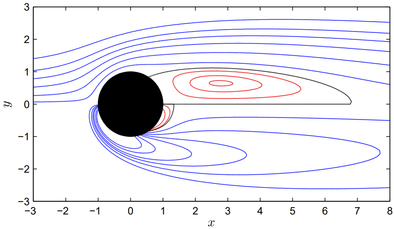
A nice way to plot both the stream function and the vorticity fields on a single graph is to plot the stream function contours for $y>0$ and the vorticity contours for $y<0$, making use of the symmetry of the fields around the $x$-axis. In way of illustration, a plot of the stream function and vorticity contours for $\operatorname{Re}=50$ is shown in Fig. 17.1.