5.5: Renormalization

Quadratic-like maps and Renormalization

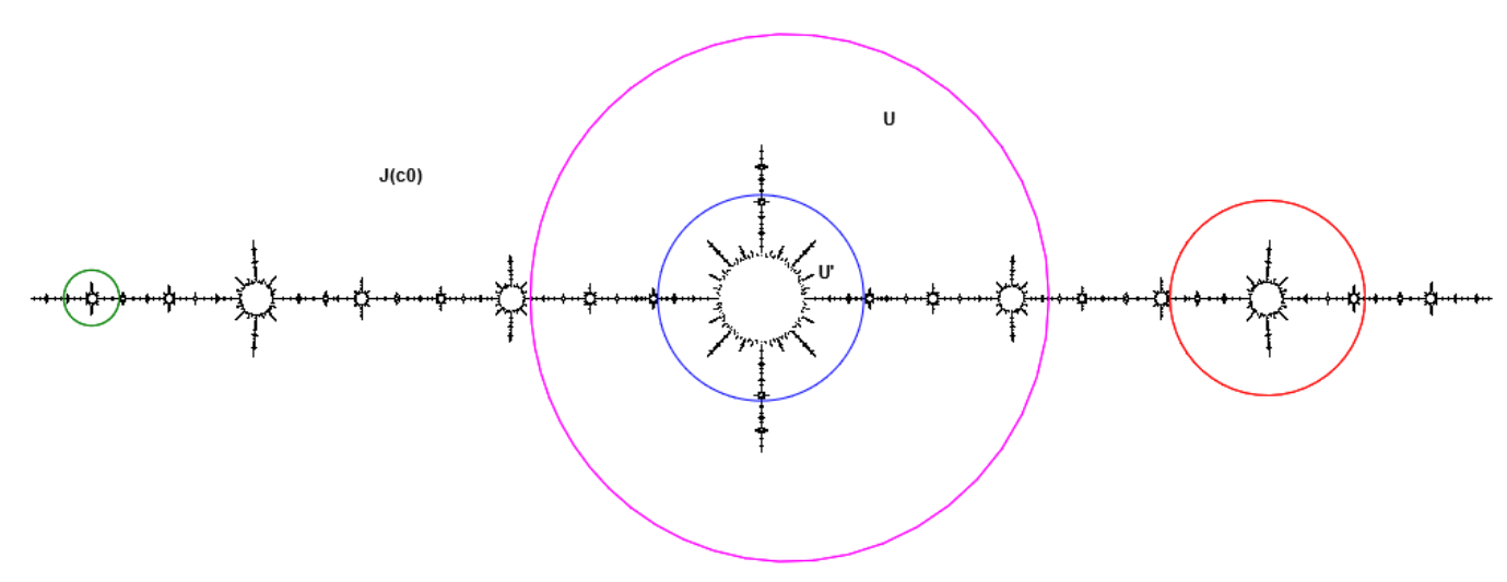
Example D Sometimes a polynomial-like map is created as some iterate of a function restricted to a domain. For example, for Q_c(z) = z² + c,   c_o ~ -1.75488 and

    U' = { |Im(z)| < 0.2, |Re(z)| < 0.2}

the polynomial Q_Co^o3 maps U' onto a larger set U with degree 2. The triple ( Q_Co^o3|_U' , U', U ) is a polynomial-like map of degree two (or quadratic-like map).

A polynomial is renormalizable if restriction of some of its iterate gives a polynomial-like map of the same or lower degree.

You see below the Mandelbrot set and a magification of its homeomorphic copy near c_o.

Figure \(\PageIndex{1}\)

For periodic point c₀ = -1.75488 with period 3 (see "airplane" below) the critical point is fixed under iterations of Q_c0^o3 therefore the filled Julia set of the quadratic-like map is homeomorphic to circle.

Figure \(\PageIndex{2}\)

For periodic point c₁ = -1.77289 with period 6 we have Q_c1^o6(0) = 0. In this case Q_c1^o3 and Q_c1^o6 are renormalizable. The critical point is periodic of period two under iterations of Q_c1^o3 therefore the filled Julia set of the quadratic-like map is homeomorphic to the Julia set z² - 1 (in square). For Q_c1^o6 the critical point is fixed so the renormalized polynomial is z² (the greatest bulb in the center)

Figure \(\PageIndex{3}\)

Figure \(\PageIndex{4}\)

Example E For c = -1.401155... the map Q_c is the Feigenbaum polynomial, that is the limit of the cascade of period doublings in the real axis. For any n the polynomial Q_c^o2n is renormalizable and all these renormalizations are hybrid equivalent to itself.

Renormalization of Q_c^o2 is shown to the left and below.

Figure \(\PageIndex{4}\)

Figure \(\PageIndex{5}\)

Figure \(\PageIndex{6}\)

Example F Let c = 0.419643 + 0.60629i is a Misiurewicz point in the boundary of the Mandelbrot set. For this map z = 0 becomes periodic of period two after three iterations (see the picture). Since Q_c^o2 is renormalizable, z = 0 is fixed after two iterations of the renormalized map. Hence, the renormilized filled Julia set is hybrid equivalent to z² - 2 , i.e. a quasiconformal image of the interval [-2, 2] (curve 2-0-4 to the left).