6.2: Misiurewicz points and the M-set self-similarity

Last updated
Save as PDF

Page ID: 102618

Robert L. Devaney

\( \newcommand{\vecs}[1]{\overset { \scriptstyle \rightharpoonup} {\mathbf{#1}} } \) \( \newcommand{\vecd}[1]{\overset{-\!-\!\rightharpoonup}{\vphantom{a}\smash {#1}}} \)\(\newcommand{\id}{\mathrm{id}}\) \( \newcommand{\Span}{\mathrm{span}}\) \( \newcommand{\kernel}{\mathrm{null}\,}\) \( \newcommand{\range}{\mathrm{range}\,}\) \( \newcommand{\RealPart}{\mathrm{Re}}\) \( \newcommand{\ImaginaryPart}{\mathrm{Im}}\) \( \newcommand{\Argument}{\mathrm{Arg}}\) \( \newcommand{\norm}[1]{\| #1 \|}\) \( \newcommand{\inner}[2]{\langle #1, #2 \rangle}\) \( \newcommand{\Span}{\mathrm{span}}\) \(\newcommand{\id}{\mathrm{id}}\) \( \newcommand{\Span}{\mathrm{span}}\) \( \newcommand{\kernel}{\mathrm{null}\,}\) \( \newcommand{\range}{\mathrm{range}\,}\) \( \newcommand{\RealPart}{\mathrm{Re}}\) \( \newcommand{\ImaginaryPart}{\mathrm{Im}}\) \( \newcommand{\Argument}{\mathrm{Arg}}\) \( \newcommand{\norm}[1]{\| #1 \|}\) \( \newcommand{\inner}[2]{\langle #1, #2 \rangle}\) \( \newcommand{\Span}{\mathrm{span}}\)\(\newcommand{\AA}{\unicode[.8,0]{x212B}}\)

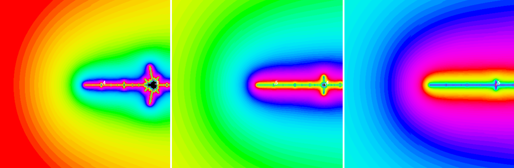
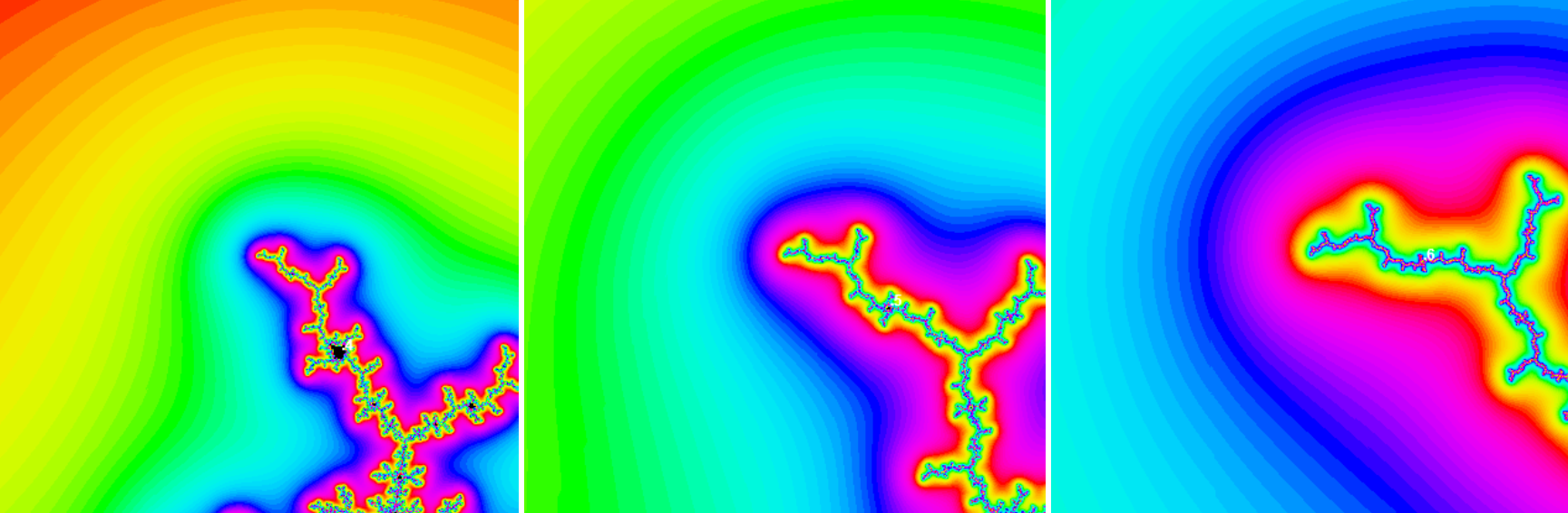
Here are illustrations of M near some of Misiurewicz points. Preperiodic points are in the center of the pictures. The images are zoomed 4, 3 and 1.328³ = 2.34 times respectevely. Some self-similar periodic points with its period are shown too.

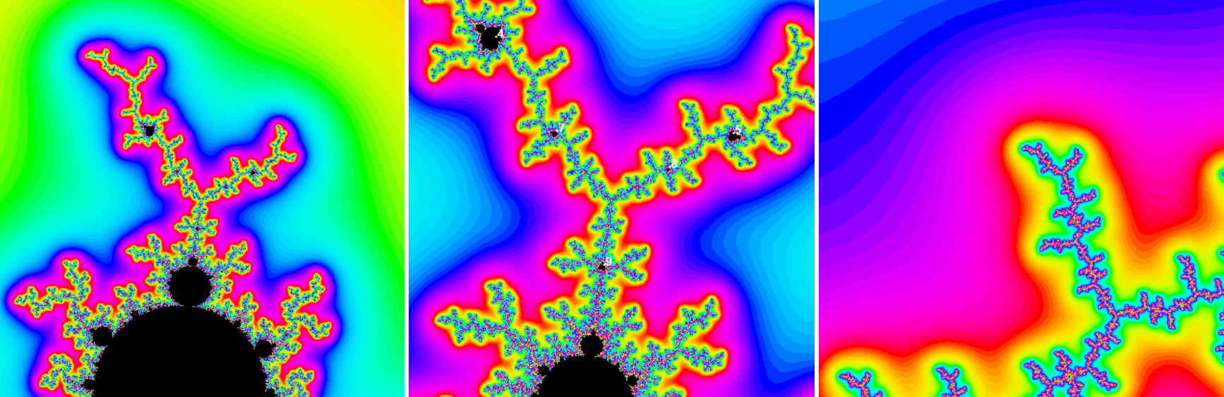
In the last figures rotational angle is very close to 120^o, which accounts for the 3-fold rotational symmetry in the picture. In the center of the picture one has 3 lines meeting, and there are numerous nearby points where 6 lines meet. At each of the letter points there is a tiny replica of M.

You see, that preperiodic points explain too spokes symmetry in the largest antenna attached to a primary bulb.

These pictures have next features in common:

The preperiodic points are not in black regions of M.
They exhibit self-similarity, i.e., they look roughly the same at shrinking the picture centered at preperiodic point by a factor of |λ| and rotating through the angle Arg(λ). This becomes more precise as the magnification increases. The rotational angles of the sequences are -23.1256^o and 119.553^o respectively. This accounts for the slight changes in orientation under successive magnifications in figures.
There is a sequence of miniature Ms of decreasing size converging to the point. Each of them has a periodic point in its main cardioid (see the theorem below). When we shrink the picture by a factor of λ the miniature Ms shrink by a factor of λ² therefore nearby miniature Ms shrink faster than the view window, so they eventually disappear.
There is a fourth feature not visible in these pictures: For preperiodic point c_o , the Julia set J(c_o) near the point z = c_o looks very much like the Mandelbrot set M near c_o. This is a theorem of Lei, which we will discuss on the next page.

Theorem Let c_o be a preperiodic point with period 1. Let c_n denote the nearest periodic point with period n. Then as n approaches infinity

(c_n - c₀ )/(c_n+1 - c₀ ) → λ = 2h

where h is the fixed point of the critical orbit of c_o .

Proof: We will use Newton's approximation to find a root of an equation f_Cn^on(0) = 0 for periodic point c_n with period n near c_o . If (c_n - c_o) value is small enough, then

f_Cn^on(0) = f_Co+(Cn-Co)^on(0) = f_Co^on(0) + (c_n - c_o) ^d/_dc f_C^on(0) |_C=Co = 0

(we do not prove that we can use this approximation). For simplicity we will denote

d_n = ^d/_dc f_C^on(0) |_C=Co .

As c_o is preperiodic with period 1, than f_Co^on(0) = h for large enough n, therefore

c_n - c_o = - h/d_n .

Since f_C^o⁽ⁿ⁺¹⁾(0) = [f_C^on(0)]² + c, it follows that for large n

d_n+1 = 2 h d_n + 1

and

(c_n - c_o )/(c_n+1 - c_o ) = (h/d_n)/(h/d_n+1) = d_n+1 /d_n = 2h + 1/d_n.

The limit of this as n approaches infinity is 2h as claimed, because d_n gets arbitrarily large for large n.