3.4E: Exercises
- Page ID
- 31085
\( \newcommand{\vecs}[1]{\overset { \scriptstyle \rightharpoonup} {\mathbf{#1}} } \)
\( \newcommand{\vecd}[1]{\overset{-\!-\!\rightharpoonup}{\vphantom{a}\smash {#1}}} \)
\( \newcommand{\id}{\mathrm{id}}\) \( \newcommand{\Span}{\mathrm{span}}\)
( \newcommand{\kernel}{\mathrm{null}\,}\) \( \newcommand{\range}{\mathrm{range}\,}\)
\( \newcommand{\RealPart}{\mathrm{Re}}\) \( \newcommand{\ImaginaryPart}{\mathrm{Im}}\)
\( \newcommand{\Argument}{\mathrm{Arg}}\) \( \newcommand{\norm}[1]{\| #1 \|}\)
\( \newcommand{\inner}[2]{\langle #1, #2 \rangle}\)
\( \newcommand{\Span}{\mathrm{span}}\)
\( \newcommand{\id}{\mathrm{id}}\)
\( \newcommand{\Span}{\mathrm{span}}\)
\( \newcommand{\kernel}{\mathrm{null}\,}\)
\( \newcommand{\range}{\mathrm{range}\,}\)
\( \newcommand{\RealPart}{\mathrm{Re}}\)
\( \newcommand{\ImaginaryPart}{\mathrm{Im}}\)
\( \newcommand{\Argument}{\mathrm{Arg}}\)
\( \newcommand{\norm}[1]{\| #1 \|}\)
\( \newcommand{\inner}[2]{\langle #1, #2 \rangle}\)
\( \newcommand{\Span}{\mathrm{span}}\) \( \newcommand{\AA}{\unicode[.8,0]{x212B}}\)
\( \newcommand{\vectorA}[1]{\vec{#1}} % arrow\)
\( \newcommand{\vectorAt}[1]{\vec{\text{#1}}} % arrow\)
\( \newcommand{\vectorB}[1]{\overset { \scriptstyle \rightharpoonup} {\mathbf{#1}} } \)
\( \newcommand{\vectorC}[1]{\textbf{#1}} \)
\( \newcommand{\vectorD}[1]{\overrightarrow{#1}} \)
\( \newcommand{\vectorDt}[1]{\overrightarrow{\text{#1}}} \)
\( \newcommand{\vectE}[1]{\overset{-\!-\!\rightharpoonup}{\vphantom{a}\smash{\mathbf {#1}}}} \)
\( \newcommand{\vecs}[1]{\overset { \scriptstyle \rightharpoonup} {\mathbf{#1}} } \)
\( \newcommand{\vecd}[1]{\overset{-\!-\!\rightharpoonup}{\vphantom{a}\smash {#1}}} \)
\(\newcommand{\avec}{\mathbf a}\) \(\newcommand{\bvec}{\mathbf b}\) \(\newcommand{\cvec}{\mathbf c}\) \(\newcommand{\dvec}{\mathbf d}\) \(\newcommand{\dtil}{\widetilde{\mathbf d}}\) \(\newcommand{\evec}{\mathbf e}\) \(\newcommand{\fvec}{\mathbf f}\) \(\newcommand{\nvec}{\mathbf n}\) \(\newcommand{\pvec}{\mathbf p}\) \(\newcommand{\qvec}{\mathbf q}\) \(\newcommand{\svec}{\mathbf s}\) \(\newcommand{\tvec}{\mathbf t}\) \(\newcommand{\uvec}{\mathbf u}\) \(\newcommand{\vvec}{\mathbf v}\) \(\newcommand{\wvec}{\mathbf w}\) \(\newcommand{\xvec}{\mathbf x}\) \(\newcommand{\yvec}{\mathbf y}\) \(\newcommand{\zvec}{\mathbf z}\) \(\newcommand{\rvec}{\mathbf r}\) \(\newcommand{\mvec}{\mathbf m}\) \(\newcommand{\zerovec}{\mathbf 0}\) \(\newcommand{\onevec}{\mathbf 1}\) \(\newcommand{\real}{\mathbb R}\) \(\newcommand{\twovec}[2]{\left[\begin{array}{r}#1 \\ #2 \end{array}\right]}\) \(\newcommand{\ctwovec}[2]{\left[\begin{array}{c}#1 \\ #2 \end{array}\right]}\) \(\newcommand{\threevec}[3]{\left[\begin{array}{r}#1 \\ #2 \\ #3 \end{array}\right]}\) \(\newcommand{\cthreevec}[3]{\left[\begin{array}{c}#1 \\ #2 \\ #3 \end{array}\right]}\) \(\newcommand{\fourvec}[4]{\left[\begin{array}{r}#1 \\ #2 \\ #3 \\ #4 \end{array}\right]}\) \(\newcommand{\cfourvec}[4]{\left[\begin{array}{c}#1 \\ #2 \\ #3 \\ #4 \end{array}\right]}\) \(\newcommand{\fivevec}[5]{\left[\begin{array}{r}#1 \\ #2 \\ #3 \\ #4 \\ #5 \\ \end{array}\right]}\) \(\newcommand{\cfivevec}[5]{\left[\begin{array}{c}#1 \\ #2 \\ #3 \\ #4 \\ #5 \\ \end{array}\right]}\) \(\newcommand{\mattwo}[4]{\left[\begin{array}{rr}#1 \amp #2 \\ #3 \amp #4 \\ \end{array}\right]}\) \(\newcommand{\laspan}[1]{\text{Span}\{#1\}}\) \(\newcommand{\bcal}{\cal B}\) \(\newcommand{\ccal}{\cal C}\) \(\newcommand{\scal}{\cal S}\) \(\newcommand{\wcal}{\cal W}\) \(\newcommand{\ecal}{\cal E}\) \(\newcommand{\coords}[2]{\left\{#1\right\}_{#2}}\) \(\newcommand{\gray}[1]{\color{gray}{#1}}\) \(\newcommand{\lgray}[1]{\color{lightgray}{#1}}\) \(\newcommand{\rank}{\operatorname{rank}}\) \(\newcommand{\row}{\text{Row}}\) \(\newcommand{\col}{\text{Col}}\) \(\renewcommand{\row}{\text{Row}}\) \(\newcommand{\nul}{\text{Nul}}\) \(\newcommand{\var}{\text{Var}}\) \(\newcommand{\corr}{\text{corr}}\) \(\newcommand{\len}[1]{\left|#1\right|}\) \(\newcommand{\bbar}{\overline{\bvec}}\) \(\newcommand{\bhat}{\widehat{\bvec}}\) \(\newcommand{\bperp}{\bvec^\perp}\) \(\newcommand{\xhat}{\widehat{\xvec}}\) \(\newcommand{\vhat}{\widehat{\vvec}}\) \(\newcommand{\uhat}{\widehat{\uvec}}\) \(\newcommand{\what}{\widehat{\wvec}}\) \(\newcommand{\Sighat}{\widehat{\Sigma}}\) \(\newcommand{\lt}{<}\) \(\newcommand{\gt}{>}\) \(\newcommand{\amp}{&}\) \(\definecolor{fillinmathshade}{gray}{0.9}\)Section Exercises
Verbal
1. What is the difference between an \(x\)-intercept and a zero of a polynomial function \(f\)?
Answer: The \(x\)-intercept is where the graph of the function crosses thex-axis, and the zero of the function is the input value for which \(f(x)=0\).
2. If a polynomial function of degree \(n\) has \(n\) distinct zeros, what do you know about the graph of the function?
3. Explain how the Intermediate Value Theorem can assist us in finding a zero of a function.
Answer: If we evaluate the function at \(a\) and at \(b\) and the sign of the function value changes, then we know a zero exists between \(a\) and \(b\).
4. Explain how the factored form of the polynomial helps us in graphing it.
5. If the graph of a polynomial just touches the \(x\)-axis and then changes direction, what can we conclude about the factored form of the polynomial?
Answer: There will be a factor raised to an even power.
Algebraic
For the following exercises, find the \(x\)-or \(t\)-intercepts of the polynomial functions.
6. \(C(t)=2(t−4)(t+1)(t−6)\)
7. \(C(t)=3(t+2)(t−3)(t+5)\)
Answer: \((−2,0),(3,0),(−5,0)\)
8. \(C(t)=4t(t−2)^2(t+1)\)
9. \(C(t)=2t(t−3)(t+1)^2\)
Answer: \((3,0),(−1,0),(0,0)\)
10. \(C(t)=2t^4−8t^3+6t^2\)
11. \(C(t)=4t^4+12t^3−40t^2\)
Answer: \((0,0), (−5,0), (2,0)\)
12. \(f(x)=x^4−x^2\)
13. \(f(x)=x^3+x^2−20x\)
Answer: \((0,0), (−5,0), (4,0)\)
14. \(f(x)=x^3+6x^2−7x\)
Exercise \(\PageIndex{15}\)
\(f(x)=x^3+x^2−4x−4\)
- Answer
-
\((2,0), (−2,0), (−1,0)\)
16. \(f(x)=x^3+2x^2−9x−18\)
17. \(f(x)=2x^3−x^2−8x+4\)
Answer: \((−2,0),(2,0),(\frac{1}{2},0)\)
18. \(f(x)=x^6−7x^3−8\)
19. \(f(x)=2x^4+6x^2−8\)
Answer: \((1,0), (−1,0)\)
20. \(f(x)=x^3−3x^2−x+3\)
21. \(f(x)=x^6−2x^4−3x^2\)
Answer: \((0,0),(\sqrt{3},0),(−\sqrt{3},0)\)
22. \(f(x)=x^6−3x^4−4x^2\)
23. \(f(x)=x^5−5x^3+4x\)
Answer: \((0,0), (1,0), (−1,0), (2,0), (−2,0)\)
For the following exercises, use the Intermediate Value Theorem to confirm that the given polynomial has at least one zero within the given interval.
24. \(f(x)=x^3−9x\), between \(x=−4\) and \(x=−2\).
25. \(f(x)=x^3−9x\), between \(x=2\) and \(x=4\).
Answer: \(f(2)=–10\) and \(f(4)=28\). Sign change confirms.
26. \(f(x)=x^5−2x\), between \(x=1\) and \(x=2\).
27. \(f(x)=−x^4+4\), between \(x=1\) and \(x=3\).
Answer: \(f(1)=3\) and \(f(3)=–77.\) Sign change confirms.
28. \(f(x)=−2x^3−x\), between \(x=–1\) and \(x=1\).
Exercise \(\PageIndex{29}\)
\(f(x)=x^3−100x+2\), between \(x=0.01\) and \(x=0.1\)
- Answer
-
\(f(0.01)=1.000001 \) and \(f(0.1)=–7.999.\) Sign change confirms.
For the following exercises, find the zeros and give the multiplicity of each.
30. \(f(x)=(x+2)^3(x−3)^2\)
31. \(f(x)=x^2(2x+3)^5(x−4)^2\)
Answer: 0 with multiplicity 2,\(−\frac{3}{2}\) with multiplicity 5, 4 with multiplicity 2
32. \(f(x)=x^3(x−1)^3(x+2)\)
33. \(f(x)=x^2(x^2+4x+4)\)
Answer: 0 with multiplicity 2, –2 with multiplicity 2
34. \(f(x)=(2x+1)^3(9x^2−6x+1)\)
Exercise \(\PageIndex{35}\)
\(f(x)=(3x+2)^5(x^2−10x+25)\)
- Answer
-
\(−\frac{2}{3}\) with multiplicity 5,5 with multiplicity 2
36. \(f(x)=x(4x^2−12x+9)(x^2+8x+16)\)
37. \(f(x)=x^6−x^5−2x^4\)
Answer: 0 with multiplicity 4,2 with multiplicity 1,–1 with multiplicity 1
38. \(f(x)=3x^4+6x^3+3x^2\)
39. \(f(x)=4x^5−12x^4+9x^3\)
Answer: \(\frac{3}{2}\) with multiplicity 2, 0 with multiplicity 3
40. \(f(x)=2x^4(x^3−4x^2+4x)\)
41. \(f(x)=4x^4(9x^4−12x^3+4x^2)\)
Answer: 0 with multiplicity 6, \frac{2}{3}\) with multiplicity 2
Graphical
For the following exercises, graph the polynomial functions. Note \(x\)- and \(y\)-intercepts, multiplicity, and end behavior.
42. \(f(x)=(x+3)^2(x−2)\)
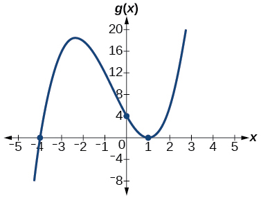
43. \(g(x)=(x+4)(x−1)^2\)
Answer: x-intercepts, \((1, 0)\) with multiplicity 2, \((–4, 0)\) with multiplicity 1, \(y\)- intercept \((0, 4)\) . As \(x→−∞\), \(f(x)→−∞\), as \(x→∞,\) \(f(x)→∞\).
44. \(h(x)=(x−1)^3(x+3)^2\)
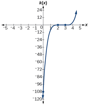
45. \(k(x)=(x−3)^3(x−2)^2\)
Answer: x-intercepts \((3,0)\) with multiplicity 3, \((2,0)\) with multiplicity 2, \(y\)- intercept \((0,–108).\) As \(x→−∞,\) \(f(x)→−∞\), as \(x→∞,\) \(f(x)→∞\).
46. \(m(x)=−2x(x−1)(x+3)\)
Exercise \(\PageIndex{47}\)
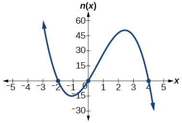
\(n(x)=−3x(x+2)(x−4)\)
- Answer
-
x-intercepts \((0, 0),(–2, 0),(4, 0)\) with multiplicity 1, y-intercept (0, 0). As \(x→−∞,\) \(f(x)→∞\), as \(x→∞,\) \(f(x)→−∞\).
For the following exercises, use the graphs to write the formula for a polynomial function of least degree.
48.
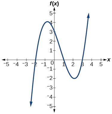
49.
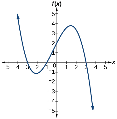
Answer: \(f(x)=−\frac{2}{9}(x−3)(x+1)(x+3)\)
50.
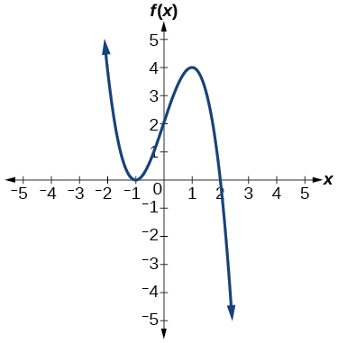
Exercise \(\PageIndex{51}\)
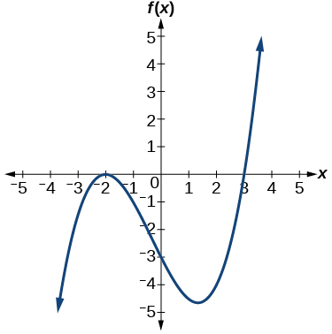
- Answer
-
\(f(x)=\frac{1}{4}(x+2)^2(x−3)\)
52.
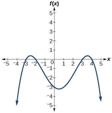
For the following exercises, use the graph to identify zeros and multiplicity.
Exercise \(\PageIndex{53}\)
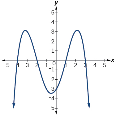
- Answer
-
–4, –2, 1, 3 with multiplicity 1
54.
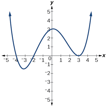
55.
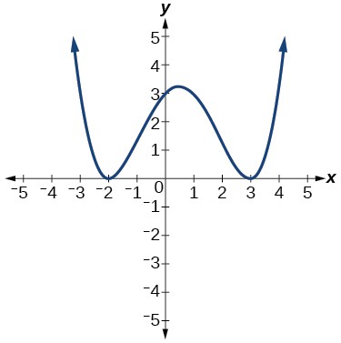
Answer: –2, 3 each with multiplicity 2
56.
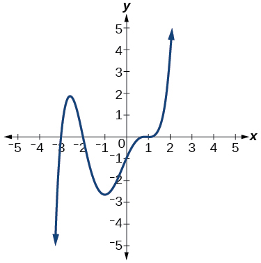
For the following exercises, use the given information about the polynomial graph to write the equation.
57. Degree 3. Zeros at \(x=–2\),\(x=1\),and \(x=3.\) y-intercept at \((0,–4)\).
Answer: \(f(x)=−\frac{2}{3}(x+2)(x−1)(x−3)\)
58. Degree 3. Zeros at \(x=–5,\) \(x=–2\),and \(x=1.\)y-intercept at \((0,6)\)
Exercise \(\PageIndex{59}\)
Degree 5. Roots of multiplicity 2 at \(x=3\) and \(x=1,\) and a root of multiplicity 1 at \(x=–3.\) y-intercept at \((0,9)\)
- Answer
-
\(f(x)=\frac{1}{3}(x−3)^2(x−1)^2(x+3)\)
60. Degree 4. Root of multiplicity 2 at \(x=4,\) and a roots of multiplicity 1 at \(x=1\) and \(x=–2.\) y-intercept at \((0,–3).\)
61. Degree 5. Double zero at \(x=1,\) and triple zero at \(x=3.\) Passes through the point \((2,15).\)
Answer: \(f(x)=−15(x−1)^2(x−3)^3\)
62. Degree 3. Zeros at \(x=4,\) \(x=3\),and \(x=2.\) y-intercept at \((0,−24).\)
63. Degree 3. Zeros at \(x=−3,\) \(x=−2\) and \(x=1.\) y-intercept at \((0,12).\)
Answer: \(f(x)=−2(x+3)(x+2)(x−1)\)
64. Degree 5. Roots of multiplicity 2 at \(x=−3\) and \(x=2\) and a root of multiplicity 1 at \(x=−2\). y-intercept at \((0, 4)\).
65. Degree 4. Roots of multiplicity 2 at \(x=\frac{1}{2}\)
and roots of multiplicity 1 at \(x=6 \) and \(x=−2.\) y-intercept at \((0,18).\)
Answer: \(f(x)=−\frac{3}{2}(2x−1)^2(x−6)(x+2)\)
66. Double zero at \(x=−3\) and triple zero at \(x=0.\) Passes through the point \((1,32).\)
Technology
For the following exercises, use a calculator to approximate local minima and maxima or the global minimum and maximum.
67. \(f(x)=x^3−x−1\)
Answer: local max \((–.58, –.62)\), local min \((.58, –1.38)\)
68. \(f(x)=2x^3−3x−1\)
69. \(f(x)=x^4+x\)
Answer: global min \((–.63, –.47)\)
70. \(f(x)=−x^4+3x−2\)
71. \(f(x)=x^4−x^3+1\)
Answer: global min \((.75, .89)\)
Extensions
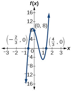
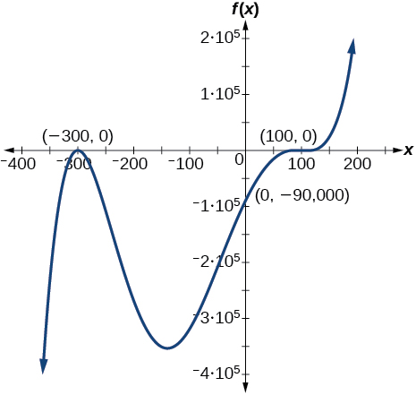
For the following exercises, use the graphs to write a polynomial function of least degree.
72.
73.
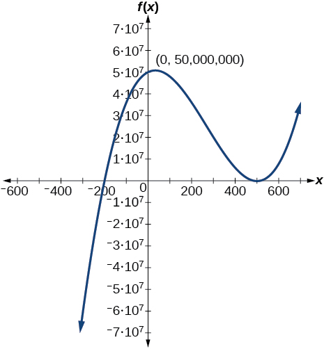
Answer: \(f(x)=(x−500)^2(x+200)\)
74.
Real-World Applications
For the following exercises, write the polynomial function that models the given situation.
Exercise \(\PageIndex{75}\)
A rectangle has a length of 10 units and a width of 8 units. Squares of \(x\) by \(x\) units are cut out of each corner, and then the sides are folded up to create an open box. Express the volume of the box as a polynomial function in terms of \(x\).
- Answer
-
\(f(x)=4x^3−36x^2+80x\)
76. Consider the same rectangle of the preceding problem. Squares of \(2x\) by \(2x\) units are cut out of each corner. Express the volume of the box as a polynomial in terms of \(x\).
77. A square has sides of 12 units. Squares \(x +1\) by \(x +1\) units are cut out of each corner, and then the sides are folded up to create an open box. Express the volume of the box as a function in terms of \(x\).
Answer: \(f(x)=4x^3−36x^2+60x+100\)
78. A cylinder has a radius of \(x+2\) units and a height of 3 units greater. Express the volume of the cylinder as a polynomial function.
79. A right circular cone has a radius of \(3x+6\) and a height 3 units less. Express the volume of the cone as a polynomial function. The volume of a cone is \(V=\frac{1}{3}πr^2h\) for radius \(r\) and height \(h\).
Answer: \(f(x)=π(9x^3+45x^2+72x+36)\)

