Search

Text Color

Margin Size

Font Type

Enable Dyslexic Font

1.7E: Exercises

Last updated

Jan 8, 2020
Save as PDF
- 1.7: Inverse Functions
- 3: Polynomial and Rational Functions

This page is a draft and is under active development.

$\newcommand{\vecs}[1]{\overset { \scriptstyle \rightharpoonup} {\mathbf{#1}} }$

$\newcommand{\vecd}[1]{\overset{-\!-\!\rightharpoonup}{\vphantom{a}\smash {#1}}}$

$\newcommand{\id}{\mathrm{id}}$ $\newcommand{\Span}{\mathrm{span}}$

( \newcommand{\kernel}{\mathrm{null}\,}\) $\newcommand{\range}{\mathrm{range}\,}$

$\newcommand{\RealPart}{\mathrm{Re}}$ $\newcommand{\ImaginaryPart}{\mathrm{Im}}$

$\newcommand{\Argument}{\mathrm{Arg}}$ $\newcommand{\norm}[1]{\| #1 \|}$

$\newcommand{\inner}[2]{\langle #1, #2 \rangle}$

$\newcommand{\Span}{\mathrm{span}}$

$\newcommand{\id}{\mathrm{id}}$

$\newcommand{\Span}{\mathrm{span}}$

$\newcommand{\kernel}{\mathrm{null}\,}$

$\newcommand{\range}{\mathrm{range}\,}$

$\newcommand{\RealPart}{\mathrm{Re}}$

$\newcommand{\ImaginaryPart}{\mathrm{Im}}$

$\newcommand{\Argument}{\mathrm{Arg}}$

$\newcommand{\norm}[1]{\| #1 \|}$

$\newcommand{\inner}[2]{\langle #1, #2 \rangle}$

$\newcommand{\Span}{\mathrm{span}}$ $\newcommand{\AA}{\unicode[.8,0]{x212B}}$

$\newcommand{\vectorA}[1]{\vec{#1}} % arrow$

$\newcommand{\vectorAt}[1]{\vec{\text{#1}}} % arrow$

$\newcommand{\vectorB}[1]{\overset { \scriptstyle \rightharpoonup} {\mathbf{#1}} }$

$\newcommand{\vectorC}[1]{\textbf{#1}}$

$\newcommand{\vectorD}[1]{\overrightarrow{#1}}$

$\newcommand{\vectorDt}[1]{\overrightarrow{\text{#1}}}$

$\newcommand{\vectE}[1]{\overset{-\!-\!\rightharpoonup}{\vphantom{a}\smash{\mathbf {#1}}}}$

$\newcommand{\vecs}[1]{\overset { \scriptstyle \rightharpoonup} {\mathbf{#1}} }$

$\newcommand{\vecd}[1]{\overset{-\!-\!\rightharpoonup}{\vphantom{a}\smash {#1}}}$

$\newcommand{\avec}{\mathbf a}$

$\newcommand{\bvec}{\mathbf b}$

$\newcommand{\cvec}{\mathbf c}$

$\newcommand{\dvec}{\mathbf d}$

$\newcommand{\dtil}{\widetilde{\mathbf d}}$

$\newcommand{\evec}{\mathbf e}$

$\newcommand{\fvec}{\mathbf f}$

$\newcommand{\nvec}{\mathbf n}$

$\newcommand{\pvec}{\mathbf p}$

$\newcommand{\qvec}{\mathbf q}$

$\newcommand{\svec}{\mathbf s}$

$\newcommand{\tvec}{\mathbf t}$

$\newcommand{\uvec}{\mathbf u}$

$\newcommand{\vvec}{\mathbf v}$

$\newcommand{\wvec}{\mathbf w}$

$\newcommand{\xvec}{\mathbf x}$

$\newcommand{\yvec}{\mathbf y}$

$\newcommand{\zvec}{\mathbf z}$

$\newcommand{\rvec}{\mathbf r}$

$\newcommand{\mvec}{\mathbf m}$

$\newcommand{\zerovec}{\mathbf 0}$

$\newcommand{\onevec}{\mathbf 1}$

$\newcommand{\real}{\mathbb R}$

$\newcommand{\twovec}[2]{\left[\begin{array}{r}#1 \\ #2 \end{array}\right]}$

$\newcommand{\ctwovec}[2]{\left[\begin{array}{c}#1 \\ #2 \end{array}\right]}$

$\newcommand{\threevec}[3]{\left[\begin{array}{r}#1 \\ #2 \\ #3 \end{array}\right]}$

$\newcommand{\cthreevec}[3]{\left[\begin{array}{c}#1 \\ #2 \\ #3 \end{array}\right]}$

$\newcommand{\fourvec}[4]{\left[\begin{array}{r}#1 \\ #2 \\ #3 \\ #4 \end{array}\right]}$

$\newcommand{\cfourvec}[4]{\left[\begin{array}{c}#1 \\ #2 \\ #3 \\ #4 \end{array}\right]}$

$\newcommand{\fivevec}[5]{\left[\begin{array}{r}#1 \\ #2 \\ #3 \\ #4 \\ #5 \\ \end{array}\right]}$

$\newcommand{\cfivevec}[5]{\left[\begin{array}{c}#1 \\ #2 \\ #3 \\ #4 \\ #5 \\ \end{array}\right]}$

$\newcommand{\mattwo}[4]{\left[\begin{array}{rr}#1 \amp #2 \\ #3 \amp #4 \\ \end{array}\right]}$

$\newcommand{\laspan}[1]{\text{Span}\{#1\}}$

$\newcommand{\bcal}{\cal B}$

$\newcommand{\ccal}{\cal C}$

$\newcommand{\scal}{\cal S}$

$\newcommand{\wcal}{\cal W}$

$\newcommand{\ecal}{\cal E}$

$\newcommand{\coords}[2]{\left\{#1\right\}_{#2}}$

$\newcommand{\gray}[1]{\color{gray}{#1}}$

$\newcommand{\lgray}[1]{\color{lightgray}{#1}}$

$\newcommand{\rank}{\operatorname{rank}}$

$\newcommand{\row}{\text{Row}}$

$\newcommand{\col}{\text{Col}}$

$\renewcommand{\row}{\text{Row}}$

$\newcommand{\nul}{\text{Nul}}$

$\newcommand{\var}{\text{Var}}$

$\newcommand{\corr}{\text{corr}}$

$\newcommand{\len}[1]{\left|#1\right|}$

$\newcommand{\bbar}{\overline{\bvec}}$

$\newcommand{\bhat}{\widehat{\bvec}}$

$\newcommand{\bperp}{\bvec^\perp}$

$\newcommand{\xhat}{\widehat{\xvec}}$

$\newcommand{\vhat}{\widehat{\vvec}}$

$\newcommand{\uhat}{\widehat{\uvec}}$

$\newcommand{\what}{\widehat{\wvec}}$

$\newcommand{\Sighat}{\widehat{\Sigma}}$

$\newcommand{\lt}{<}$

$\newcommand{\gt}{>}$

$\newcommand{\amp}{&}$

$\definecolor{fillinmathshade}{gray}{0.9}$

Section Exercises

Verbal

Exercise 1.7.1

Describe why the horizontal line test is an effective way to determine whether a function is one-to-one?

Answer:: Each output of a function must have exactly one output for the function to be one-to-one. If any horizontal line crosses the graph of a function more than once, that means that $y$ -values repeat and the function is not one-to-one. If no horizontal line crosses the graph of the function more than once, then no $y$ -values repeat and the function is one-to-one.

Exercise 1.7.2

Why do we restrict the domain of the function $f(x)=x^2$ to find the function’s inverse?

Exercise 1.7.3

Can a function be its own inverse? Explain.

Answer:: Yes. For example, $f(x)=\frac{1}{x}$ is its own inverse.

Exercise 1.7.4

Are one-to-one functions either always increasing or always decreasing? Why or why not?

Exercise 1.7.5

How do you find the inverse of a function algebraically?

Answer:: Given a function $y=f(x)$ , solve for $x$ in terms of $y$ . Interchange the $x$ and $y$ . Solve the new equation for $y$ . The expression for $y$ is the inverse, $y=f^{-1}(x)$ .

Algebraic

Exercise 1.7.6

Show that the function $f(x)=a−x$ is its own inverse for all real numbers $a$ .

For the following exercises, find $f^{-1}(x)$ for each function.

Exercise 1.7.7

$f(x)=x+3$

Answer:: $f^{-1}(x)=x−3$

Exercise 1.7.8

$f(x)=x+5$

Exercise 1.7.9

$f(x)=2−x$

Answer:: $f^{-1}(x)=2−x$

Exercise 1.7.10:

$f(x)=3−x$

Exercise 1.7.11

$f(x)=\frac{x}{x+2}$

Answer:: $f^{-1}(x)=\frac{−2x}{x−1}$

Exercise 1.7.12

$f(x)=\frac{2x+3}{5x+4}$

For the following exercises, find a domain on which each function $f$ is one-to-one and non-decreasing. Write the domain in interval notation. Then find the inverse of $f$ restricted to that domain.

Exercise 1.7.13

$f(x)=(x+7)^2$

Answer:: domain of $f(x)$ : $\left[−7,\infty\right)$ ; $f^{-1}(x)=\sqrt{x}−7$

Exercise 1.7.14

$f(x)=(x−6)^2$

Exercise 1.7.15

$f(x)=x^2−5$

Answer:: domain of $f(x)$ : $\left[0,\infty\right)$ ; $f^{-1}(x)=\sqrt{x+5}$

Exercise 1.7.16

Given $f(x)=\frac{x}{2+x}$ and $g(x)=\frac{2x}{1-x}:$

a. Find $f(g(x))$ and $g(f(x))$ .

b. What does the answer tell us about the relationship between $f(x)$ and $g(x)?$

Answer:: a. $f(g(x))=x$ and $g(f(x))=x$ .

b. This tells us that $f$ and $g$ are inverse functions

For the following exercises, use function composition to verify that $f(x)$ and $g(x)$ are inverse functions.

Exercise 1.7.17

$f(x)=\sqrt[3]{x-1}$ and $g(x)=x^3+1$

Answer:: $f(g(x))=x$ , $g(f(x))=x$

Exercise 1.7.18

$f(x)=−3x+5$ and $g(x)=\frac{x-5}{-3}$

Graphical

For the following exercises, use a graphing utility to determine whether each function is one-to-one.

Exercise 1.7.19

$f(x)=\sqrt{x}$

Answer:: one-to-one

Exercise 1.7.20

$f(x)=\sqrt[3]{3x+1}$

Exercise 1.7.21

$f(x)=−5x+1$

Answer:: one-to-one

Exercise 1.7.22

$f(x)=x^3−27$

For the following exercises, determine whether the graph represents a one-to-one function.

Exercise 1.7.23

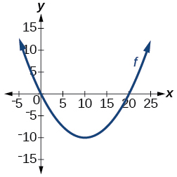
$Graph of a parabola.$

Answer:: not one-to-one

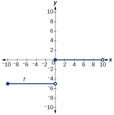
Exercise 1.7.24

$Graph of a step-function.$

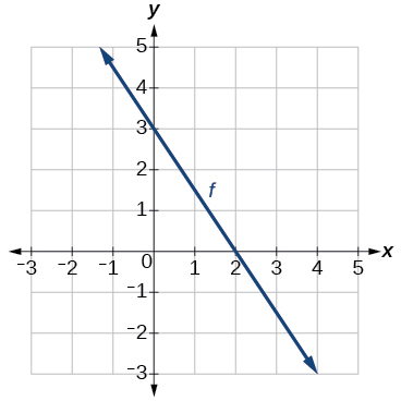
For the following exercises, use the graph of $f$ shown in Figure 1.7.11.

$Graph of a line.$

Figure 1.7.11: Graph of a line

Exercise 1.7.25

Find $f(0)$ .

Answer:: 3

Exercise 1.7.26

Solve $f(x)=0$ .

Exercise 1.7.27

Find $f^{-1}(0)$ .

Answer:: 2

Exercise 1.7.28

Solve $f^{-1}(x)=0$ .

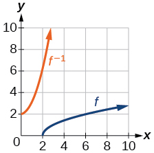
For the following exercises, use the graph of the one-to-one function shown in Figure 1.7.12.

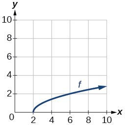
$Graph of a square root function.$
Figure 1.7.12: Graph of a square root function.

Exercise 1.7.29

Sketch the graph of $f^{-1}$ .

Answer:: $Graph of a square root function and its inverse.$

Exercise 1.7.30

Find $f(6)$ and $f^{-1}(2)$ .

Exercise 1.7.31

If the complete graph of $f$ is shown, find the domain of $f$ .

Answer:: $[2,10]$

Exercise 1.7.32

If the complete graph of $f$ is shown, find the range of $f$

Numeric

For the following exercises, evaluate or solve, assuming that the function $f$ is one-to-one.

Exercise 1.7.33

If $f(6)=7$ , find $f^{-1}(7)$ .

Answer:: 6

Exercise 1.7.34

If $f(3)=2$ , find $f^{-1}(2)$ .

Exercise 1.7.35

If $f^{-1}(−4)=−8$ , find $f(−8)$ .

Answer:: -4

Exercise 1.7.36

If $f^{-1}(−2)$ =−1, find $f(−1)$ .

For the following exercises, use the values listed in Table 1.7.6 to evaluate or solve.

$x$	$f(x)$
0	8
1	0
2	7
3	4
4	2
5	6
6	5
7	3
8	9
9	1

Table 1.7.6

Exercise 1.7.37

Find $f(1)$ .

Answer:: 0

Exercise 1.7.38

Solve $f(x)=3$ .

Exercise 1.7.39

Find $f^{-1}(0)$ .

Answer:: 1

Exercise 1.7.40

Solve $f^{-1}(x)=7$ .

Exercise 1.7.41

Use the tabular representation of $f$ in Table 1.7.7 to create a table for f^{-1}(x).

$x$	3	6	9	13	14
$f(x)$	1	4	7	12	16

Table 1.7.7

Answer:

$x$	1	4	7	12	16
$f^{-1}(x)$	3	6	9	13	14

Technology

For the following exercises, find the inverse function. Then, graph the function and its inverse.

Exercise 1.7.42

$f(x)=\dfrac{3}{x-2}$

Exercise 1.7.43

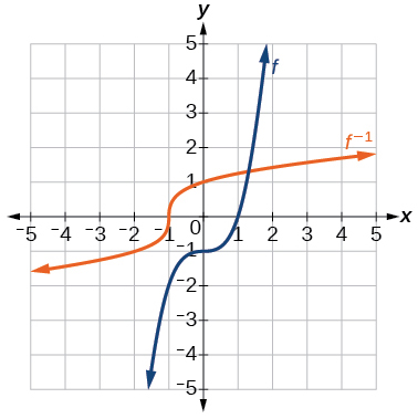
$f(x)=x^3−1$

Answer:

$f^{-1}(x)=(1+x)^{1/3}$

$Graph of a cubic function and its inverse.$

Exercise 1.7.44

Find the inverse function of $f(x)=\frac{1}{x-1}$ . Use a graphing utility to find its domain and range. Write the domain and range in interval notation.

Real-World Applications

Exercise 1.7.45

To convert from $x$ degrees Celsius to $y$ degrees Fahrenheit, we use the formula $f(x)=\frac{9}{5}x+32$ . Find the inverse function, if it exists, and explain its meaning.

Answer:: $f^{-1}(x)=\frac{5}{9}(x−32)$ . Given the Fahrenheit temperature, $x$ , this formula allows you to calculate the Celsius temperature.

Exercise 1.7.46

The circumference $C$ of a circle is a function of its radius given by $C(r)=2{\pi}r$ . Express the radius of a circle as a function of its circumference. Call this function $r(C)$ . Find $r(36\pi)$ and interpret its meaning.

Exercise 1.7.47

A car travels at a constant speed of 50 miles per hour. The distance the car travels in miles is a function of time, $t$ , in hours given by $d(t)=50t$ . Find the inverse function by expressing the time of travel in terms of the distance traveled. Call this function $t(d)$ . Find $t(180)$ and interpret its meaning.

Answer:: $t(d)=\frac{d}{50}$ , $t(180)=\frac{180}{50}$ . The time for the car to travel 180 miles is 3.6 hours.

Section Exercises

Support Center

How can we help?